2. Formulas and Functions
So far we’ve used Excel basically as a way to input, arrange and format static information. But a spreadsheet comes alive through the use of formulas and functions. As the name suggests, formulas basically correspond to some instructions that tell Excel how to combine information (numerical or text-based) into a result (e.g., 1 + 1 = 2). Functions use some built-in procedures to apply more complicated transformations (e.g., sqrt(4) = 2).
Basic Formulas
Let’s say we have information about the sales of a software package for 1998 and 1999, separately for the Eastern and Western sales region. The software has sold for $200 in both years and in both markets (see the following figure and the Software worksheet in the Intro to Excel workbook).
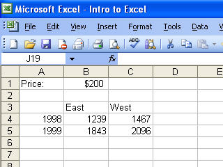
Figure 2‑1
The company would like to know the total sales for each region (over the two years) and for each year (over the two regions). Let’s look at three different ways that this can be done.
- In cell B6 type =B4+B5. Of course, this formula will give us the total sales for the Eastern sales region.
Note: Every formula and function in Excel starts with an “=” sign!
- Click on C6
and click on the AutoSum
button (
 )
in the Standard toolbar. Excel automatically pastes the SUM function into
cell C6 and selects the range C4:C5 as the arguments for this function.
Press Enter.
)
in the Standard toolbar. Excel automatically pastes the SUM function into
cell C6 and selects the range C4:C5 as the arguments for this function.
Press Enter.
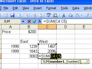
Figure 2‑2
- In cell D4 type =SUM(B4:C4) to calculate the total sales for 1998.
- With cell D4 selected, drag the AutoFill handle (the small square in the lower right hand corner of D4) down to cell D5. This is a quick way to copy formulas and functions. Excel automatically adjusts the arguments to account for the new position. In other words: since we copied the formula down to row 5, Excel adjusted the argument range from B4:C4 to B5:C5. This happens whenever we use what is called relative references to cells.
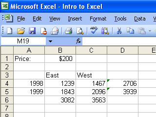
Figure 2‑3
Let’s calculate total revenues for each year.
- In cell E4 type =B1*D4 to calculate the total revenues for year 1998.
- Copy the formula from E4 to E5 (use AutoFill feature or the copy/paste commands from the Edit menu or from the Standard toolbar).
Oops. Cell E5 shows a total revenue of $0 for 1999. We know that this can’t be true. Since we used relative cell referencing in the copying process, Excel adjust the formula to =B2*D5 and of course there is no information in cell B2. We need to use absolute references to cell B1 to make sure that it won’t be changed once we copy the formula from D4 to D5.
- Go back to cell D4 and change the formula to =$B$1*D4 (one quick way to do this is to click on the B1 part in the existing formula in the formula bar and pressing the F4 key).
- Now copy the formula down to D5 to get the total sales for 1999.
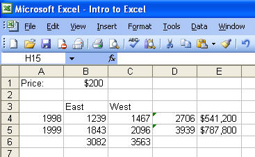
Figure 2‑4
Note: You can mix absolute and relative references. For example, since we only changed the row position in the copying process, we just need to make sure that the formula always refers to row 1. The formula =B$1*D4 would have done the trick.
Let’s assume that the goal for each year was to exceed $750,000 in total revenue. We’ll use Excel’s =IF() function to alert us whether we did or did not achieve that goal.
- In cell F4 type =IF(E4>750000,”No Need to Panic”,“Panic”) and press Enter.
The =IF() function takes three arguments: the first one is a condition that either evaluates to be true or false; the second argument gives the result if the condition is true, the third argument gives the result if the condition is false. Since the value in E4 is less than $750,000, the condition is false and Excel will report “Panic” as a result.
- Copy the formula from E4 to E5. Your worksheet should now look like this:

Figure 2‑5
Using Functions
Let’s say we wanted to calculate the average sales for each
region. Excel has hundreds for built-in functions, ranging from simple
arithmetic operations to fairly sophisticated financial and statistical
functions. You can access these functions either by choosing Insert Þ Function … or by clicking on the Paste Function button (![]() ) on next to the
formula bar.
) on next to the
formula bar.
- Select cell B7
and click on the Paste
Function button (
 ).
). - In the Insert Function dialog box, select Statistical from the Or select a category: listbox. This list gives you an idea of the wide variety of functions built into Excel.
- In the Select a function: listbox select AVERAGE.
Note: Excel offers a brief description of the selected function, including its required arguments. For more help, click on the help link in the lower left-hand corner.
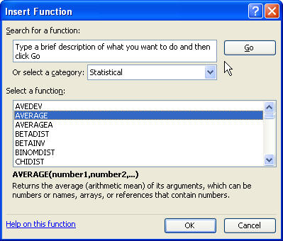
Figure 2‑6
- Click the OK button.
Excel now opens a dialog that allows you to specify the arguments for the AVERAGE function. As you can see in the following Figure, Excel “looked around” in the neighborhood of B7 to find numbers to average. We need to change that since we only want to average the two sales figures in B4 and B5.
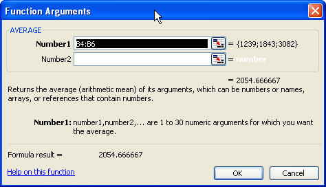
Figure 2‑7
- You can change the range in the Number1 box directly to B4:B5 or you can
click on the Collapse
Dialog button (
 )
to minimize the dialog box and get access to your spreadsheet (where you
can highlight the range from B4:B5
to supply the correct arguments; click on the Return to Dialog button
)
to minimize the dialog box and get access to your spreadsheet (where you
can highlight the range from B4:B5
to supply the correct arguments; click on the Return to Dialog button  to get back to
the dialog box).
to get back to
the dialog box). - Click the OK button.
Your worksheet now shows the average sales for the Eastern region in cell B7.
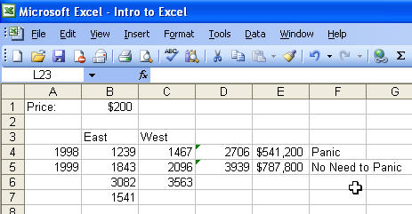
Figure 2‑8
Exercise
Use the =PMT(rate, nper, pv, fv, type) function to set up a mortgage payment calculator as shown in the following figure. The =PMT() function is available from the Financial functions and you only need to specify the first three parameters. Use Help if you need more information.
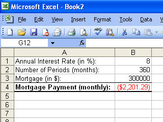
Figure 2‑9