All-to-all propagation in sensor networks using network coding

Emin Gabrielyan

2006-07-24

Abstract 1

1. Introduction. 1

2. Node level re-transmission algorithm.. 3

3. Examples of propagation of messages. 5

4. Simulations. 8

5. Reducing the overall number of network transmissions without network coding. 10

6. Conclusions. 12

References. 12

Table of figures. 13

Abstract

All-to-all communication in a sensor or ad-hoc network can be carried out by re-transmitting at each node all freshly arrived messages. In a connected network with N sensor nodes this method results in transmissions. In network coding paradigm the nodes not only re-transmit the received messages but can also transmit their linear combinations. By doing so, all-to-all communication can be carried out with a fewer number of transmissions. We propose a node level retransmission algorithm. By default the node re-transmits each piece of the fresh information linearly combined at random with the previously received information. To reduce the number of transmissions the node can sometimes linearly combine two pieces of freshly received information and send them in single transmissions. The overall number of network transmissions depends on how frequently the nodes combine two transmissions into single ones. Reduction of the overall number of network transmissions is achieved at the cost of undelivered messages. On networks with an average link density of 10% to 15%, our node-level retransmission algorithm permits to reduce the overall number of network transmissions by 50% at the cost of less than 1% undelivered messages.

1. Introduction

Network coding is an emerging area that re-examines fundamental principles of network information flow. The main idea is that we allow intermediate nodes in a network to not only forward but also to process the incoming information flows [Ahlswede00]. This simple idea promises to have a significant impact in diverse areas that include multicasting, network monitoring, reliable delivery, resource sharing, efficient flow control and security. The use of network coding techniques allows to realize benefits in terms of throughput, energy efficiency, and robustness in applications such as information dissemination in overlay networks, fixed or mobile ad-hoc wireless and sensor networks [Lun06], [Pakzad05], [Tuninetti05].

We are addressing the problem of information dissemination in an ad-hoc network. Each node in the network has a message which should be propagated to all other nodes. The simplest way is to program each node to retransmit every received fresh packet. The 3-node example shown in Figure 1 to Figure 4 requires five transmissions to deliver the messages from all nodes to all other nodes.

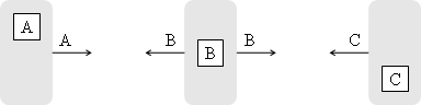
Figure 1. Three nodes initially containing a single message are broadcasting their messages to the neighbor nodes (three transmissions)

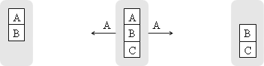
Figure 2. The middle node retransmits the message A (one transmission)

Figure 3. The middle node retransmits the message B (one transmission)

Figure 4. After five transmissions all nodes have messages of all other nodes

Figure 5 shows that the two transmissions of Figure 2 and Figure 3 can be replaced by a single transmission and the all-to-all communication can be carried out with 4 network transmissions instead of 5.

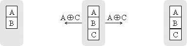
Figure 5. One transmission of an XOR packet at the middle node can replace two transmissions of Figure 2 and Figure 3

For a general case Fragouli proposed the following packet coding scheme: the coding node has a fixed, finite memory in which it stores packets formed from an incoming packet stream, and it sends packets formed from random linear combinations of its memory contents [Lun06]. The main contribution of this work is determining the conditions for a node to transmit. If the channels are erasure-less the node transmits with a probability of , every time a fresh packet is received. If the received packet is not fresh it is simply ignored and no action is taken.

We propose a method, in which the node keeps only as many checksum packets as there are source messages. The node constantly improves the stored checksum packets. As new checksum packets arrive, the node tries to partially solve the “equations” represented by all available checksum packets. At each clock cycle the node re-transmits obligatorily the fresh information retrieved from the receptions at the previous clock cycles. The node also adds at random some linear combinations of old information.

In our method we ensure that the information delivered by the fresh packets is retransmitted immediately at the next clock cycle. In order to avoid accidental cleaning of fresh information in retransmitted packets, we maximally diagonalize the matrix of received checksum packets.

The document is organized as follows. Section 2 presents the algorithm for updating the checksums of a node upon reception of new packets and the node’s retransmission strategy. Section 3 presents visualized diagrams showing the progress of the propagation of the messages according to network coding and simple retransmission algorithms. Simulation results are presented in Sections 4 and 5.

2. Node level re-transmission algorithm

Given is a network of nodes. Each node has its own message which should be propagated to all other nodes across the network. According to our model at each clock cycle all nodes are transmitting (i.e. broadcasting to their neighbors) all their queued messages. We are abstracting from the link layer implementation of simultaneous transmissions (e.g. code, time or frequency division multiplexing). The node forms its transmission queue, based on information received at the previous clock cycle. The transmission queue is not affected by the messages received at the current clock cycle.

According to a simple retransmission model, the nodes are always transmitting the original source messages without modifying them. Each received fresh message is retransmitted once at the next clock cycle. After several clock cycles all nodes ultimately receive the messages from all other nodes (if the network is connected).

In the network coding version, the node keeps a square matrix, where each row is a binary vector representing an available checksum-packet that is a linear combination of source packets. Initially the matrix consist of only zeroes except at the position . The i-th row of the matrix corresponds to the own message of the node.

During the whole time, the matrix is always maintained such that its lower triangle contains only zeroes. This is achieved by replacing the new checksum-packets with their linear combination with the existing checksum-packets (i.e. rows). It is assumed that the node has already information on the source packets for all positions of the matrix diagonal which are set to 1. When a new checksum packet arrives, the receiver cleans from that packet the already known source packets. The first non-zero component of the resulting checksum packet specifies the position of this packet in the matrix (the vector is positioned at a row where the first 1 is positioned in the diagonal). In this case, it is considered that the checksum packet delivered information on the source packet (corresponding to the new row in the matrix). If after cleaning process, the arrived checksum packets became empty, it means that it is linearly dependent and carries no new information.

At each clock cycle each node receives several checksum packets. Therefore the node collects fresh information on certain number of source packets. The rows corresponding to the fresh source packets determine the checksum packets to be transmitted by the node itself at the next clock cycle.

The node transmits a linear combination of one or two fresh rows with some old rows taken at random. Each fresh row is considered one time. Therefore, if there were n fresh rows, there will be between and n transmissions.

By transmitting a new checksum (to the next hop in the network), there is a risk that the fresh source packet component in the vector is cleaned due to linear combination with other rows. In such case the propagation of the fresh packet across the network may be delayed or even interrupted. To avoid the accidental cleaning of the fresh component in retransmitted checksums, we clean not only the lower triangle of the node’s matrix but also its upper triangle (whenever it is possible, i.e. whenever 1s are available at the diagonals).

This process is very similar to the Gaussian elimination, except that it is carried out on the fly upon the reception of every new “equation”, i.e. upon reception of every new checksum packet. The matrix update algorithm can be summarized by a short C++ code below, where N is the number of nodes in the network, m is an square matrix and c is the vector representing the received checksum.

int Decoder::insert()

{

int fresh=-1;

try

{

for(int i=0;i<N;)

{

for(;i<N && m[i][i];i++)

if(c[i])

for(int j=i;j<N;j++)

c[j]^=m[i][j];

for(;i<N && !m[i][i];i++)

if(c[i])

throw i;

}

catch(int i)

{

for(int j=i;j<N;j++)

m[i][j]=c[j];

for(int j=i;j<N;j++)

if(m[j][j])

for(int k=0;k<j;k++)

if(m[k][j])

for(int l=j;l<N;l++)

m[k][l]^=m[j][l];

fresh=i;

rank++;

}

total++;

return fresh;

}

Below is an example where a node maintains an matrix and receives sequentially eight random checksum packets. Initially the matrix is completely empty. Each new checksum packet c adds a 1 in the diagonal of the matrix m (if it contains fresh information) or is ignored (if it is linearly dependent on the rows of the matrix m) (See the output [log] and the code [zip]).

c[8]={

0 1 1 0 1 0 0 0

};

m[8][8]={

- - - - - - - -

- 1 1 - 1 - - -

- - - - - - - -

};

Source packet 1

c[8]={

0 0 1 1 1 1 1 0

};

m[8][8]={

- - - - - - - -

- 1 - 1 - 1 1 -

- - 1 1 1 1 1 -

- - - - - - - -

};

Source packet 2

c[8]={

1 0 0 1 0 1 1 0

};

m[8][8]={

1 - - 1 - 1 1 -

- 1 - 1 - 1 1 -

- - 1 1 1 1 1 -

- - - - - - - -

};

Source packet 0

c[8]={

0 0 1 1 0 0 1 1

};

m[8][8]={

1 - - 1 - 1 1 -

- 1 - 1 - 1 1 -

- - 1 1 - - 1 1

- - - - - - - -

- - - - 1 1 - 1

- - - - - - - -

};

Source packet 4

c[8]={

1 0 0 1 0 0 0 0

};

m[8][8]={

1 - - 1 - - - -

- 1 - 1 - - - -

- - 1 1 - - 1 1

- - - - - - - -

- - - - 1 - 1 1

- - - - - 1 1 -

- - - - - - - -

};

Source packet 5

c[8]={

0 1 1 0 0 0 1 1

};

m[8][8]={

1 - - 1 - - - -

- 1 - 1 - - - -

- - 1 1 - - 1 1

- - - - - - - -

- - - - 1 - 1 1

- - - - - 1 1 -

- - - - - - - -

};

No fresh info

c[8]={

1 1 1 0 0 0 1 1

};

m[8][8]={

1 - - - - - - -

- 1 - - - - - -

- - 1 - - - 1 1

- - - 1 - - - -

- - - - 1 - 1 1

- - - - - 1 1 -

- - - - - - - -

};

Source packet 3

c[8]={

0 1 0 1 0 0 0 1

};

m[8][8]={

1 - - - - - - -

- 1 - - - - - -

- - 1 - - - 1 -

- - - 1 - - - -

- - - - 1 - 1 -

- - - - - 1 1 -

- - - - - - - -

- - - - - - - 1

};

Source packet 7

c[8]={

0 0 0 0 1 0 1 1

};

m[8][8]={

1 - - - - - - -

- 1 - - - - - -

- - 1 - - - 1 -

- - - 1 - - - -

- - - - 1 - 1 -

- - - - - 1 1 -

- - - - - - - -

- - - - - - - 1

};

No fresh info

c[8]={

1 1 1 1 1 1 0 0

};

m[8][8]={

1 - - - - - - -

- 1 - - - - - -

- - 1 - - - - -

- - - 1 - - - -

- - - - 1 - - -

- - - - - 1 - -

- - - - - - 1 -

- - - - - - - 1

};

Source packet 6

3. Examples of propagation of messages

The Figure 6 and Figure 7 present different stages of the propagation of information in network. The both figures show in parallel the progress of two algorithms: the simple fresh-message-retransmission algorithm and the network coding algorithm. The amount of fresh information collected by each node according to the first and second algorithms is shown by two semicircles. The outer red semicircle shows the number of messages delivered according to the first simple algorithm and the inner green semicircle shows the number of messages delivered according the second network coding algorithm. The number on the node corresponds only to the number of messages received according the firs simple algorithm. Figure 6 shows that initially each node contains only one message, at this moment there are total 20 fresh messages in the network (according both algorithms), there are already 20 messages delivered (according to initial condition) and there are no carried out transmissions yet.

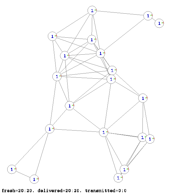
Figure 6. The initial state of the network where each node contains only 1 message (its own). The colon separated records at the bottom of the figure indicate on the number of freshly received packets by all nodes in the network, on the overall number of delivered packets in the network and on the total number of transmissions. The first number (before the colon) corresponds to the simple re-transmission algorithm and the second number (after the colon) corresponds to our network coding algorithm.

Figure 7 shows that after three transmission clock cycles the first simple retransmission algorithm delivered 348 messages with 238 transmissions and the second network coding algorithm delivered a slightly fewer number of message (311) but with a much less number of network transmissions (134).

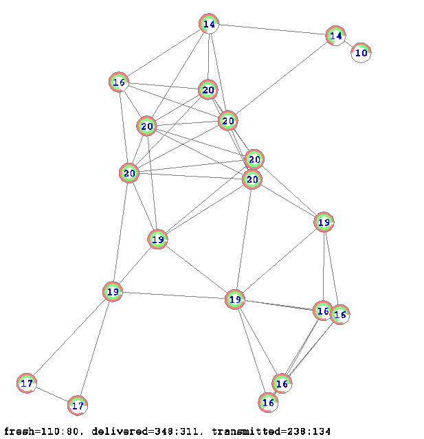
Figure 7. The diagram shows the state of the network after three transmission clock cycles. The red (outer) semi-circled sector at node shows the percentage of the messages collected by the node by using the simple message re-transmission method. The green (inner) sector shows the percentage of the useful information collected by the node (i.e. the rank of the matrix) according to the network coding method. The numbers shown on the nodes correspond to the messages received by the simple re-transmission algorithm (the outer semi-circle).

The animated version of the propagation process by both algorithms is shown in Figure 8. The figure shows in parallel propagation of messages by the two algorithms. The propagation is shown for six different network samples.

Figure 8. Propagation of the messages across the network through two algorithms for six random network samples [gif], [pdf], [ps], [log] (the C++ codes [zip])

4. Simulations

We are evaluating the efficiency of our network coding algorithm by measuring the delivery ratio (fraction of nodes collecting all messages) as a function of reduction in the number of transmissions (achieved by combining at random the fresh messages into single transmissions). Reduction in the overall number of transmissions is measured as a fraction of the total number of transmissions required by the flooding algorithm individually re-transmitting all fresh messages.

By increasing the rate of linear coupling of pairs of fresh checksums we reduce the overall number of transmissions. One simulation event results in a number of network transmissions and in an overall delivery ratio. We generated 20’000 simulation results. Figure 9 shows that most of the time a delivery to all nodes is ensured even by reducing the overall number of network transmissions by half.

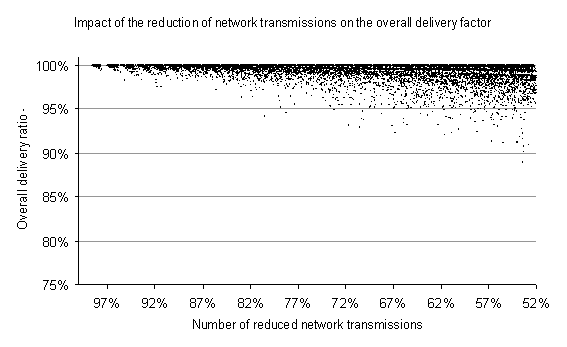
Figure 9. Simulations on 20,000 randomly generated network samples using our network coding algorithm [csv]

Figure 10 shows that in average by reducing the overall number of network transmissions by half the damage caused to the delivery ratio do not exceed 1%.

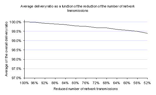
Figure 10. Average delivery ratio as a function of the reduction of network transmissions [xls]

The number of nodes is 80 in all network samples. The link density (in respect to fully connected graphs) varies from 10% to 15%. The network samples are obtained by randomly throwing the nodes on a rectangular area of size and by connecting the nodes that are sufficiently close to each other (according to the coverage radius of the nodes). The coverage radius of the nodes is computed as follows:

(1)

The coefficient c is equal for all our samples to 3.5. Higher this coefficient denser the network is.

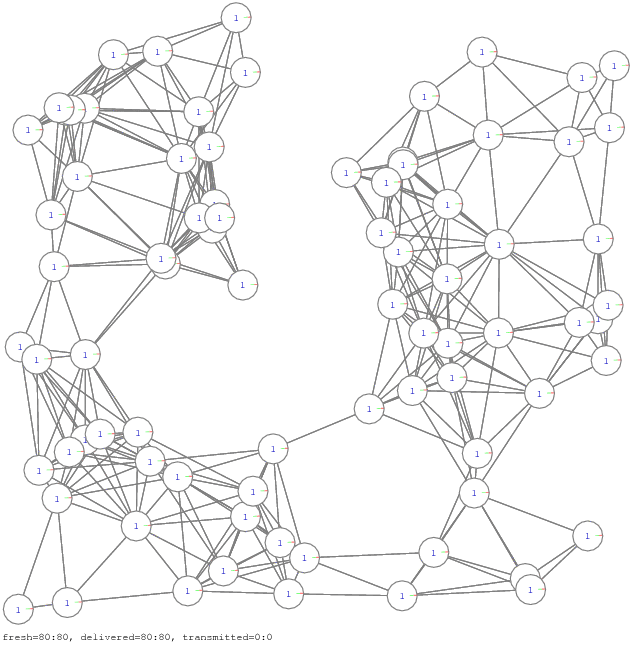
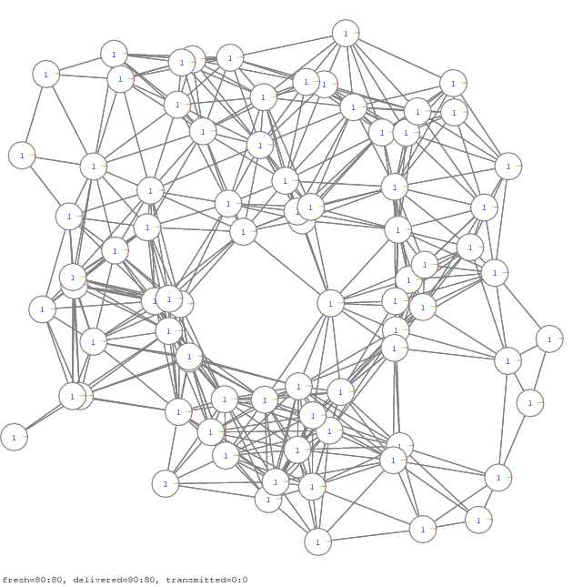
The simulator is a small C++ program [zip] of about thousand lines. Figure 11 and Figure 12 show few network samples used in the simulation. For visualization, the simulator generates initially postscript files. They are converted to PDF and GIF files using respectively AFPL Ghostscript and ImageMagick freeware packages.

Figure 11. Propagation of all-to-all communication on 12 network samples [pdf], [gif], [ps]

Figure 12. Propagation of all-to-all communication, another example of 12 network samples [pdf], [gif], [ps]

The impact of the reduction of the overall number of network transmissions to the overall delivery ratio depends on the density of the links in the network. Logically the impact is more if the density is low, i.e. when the coefficient c in equation (1) is small.

5. Reducing the overall number of network transmissions without network coding

Even with a simple re-transmission algorithm there is a certain probability that the messages will be still delivered when the nodes are simply skipping re-transmissions of fresh messages, randomly at a low rate. By skipping re-transmissions, the number of transmissions in the network is reduced. The impact on the overall delivery ratio is minimal when the network is dense and the delivery of messages from their sources to their destinations is possible through numerous independent paths.

Overall delivery ratio as a function of the reduction in the number of network transmissions is computed for such a simple method using 10’000 simulation samples. The network samples are generated with the same number of nodes and link density as used for the simulations of section 4 (with network coding). Figure 13 shows that compared with the network coding algorithm (see Figure 9), in the retransmission-skipping method the reduction in the number of network transmissions is achieved at a much higher cost of undelivered messages.

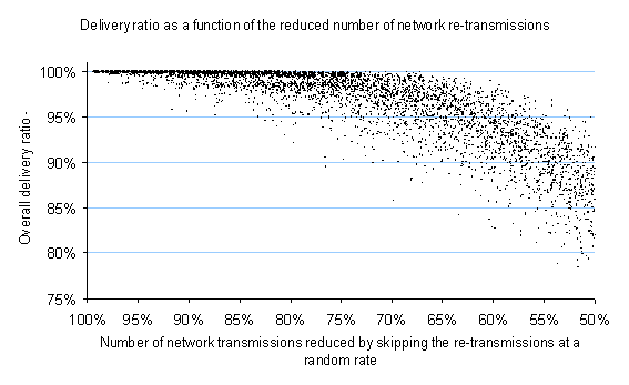
Figure 13. Impact of the skipped re-transmissions to the overall delivery ratio in a simple fresh message re-transmission mode [csv], [xls]

The simulator is a small C++ program [zip]. The propagation diagrams comparing the two message retransmission methods, with and without skipping of retransmissions, are shown in Figure 14.

Figure 14. Propagation of messages by simple re-transmissions with and without skipping of re-transmissions [pdf], [gif], [ps]

Finally, the comparison of the average delivery ratios of the network coding method and of the retransmission skipping method is given in a chart of Figure 15.

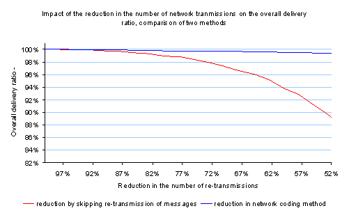
Figure 15. Comparison of the overall delivery ratios of the network coding method and skipped retransmissions method

In order to make the skipped retransmissions method not too bad, we “oblige” each node at each clock cycle to re-transmit at least one fresh message. In such a way we ensure that for example at the first clock cycle, all nodes will transmit obligatorily their source messages and there is no risk that a source message will be lost at the first clock cycle for all other nodes. Figure 15 shows that even with this little improvement the skipped re-transmissions method is significantly worst than the network coding method.

6. Conclusions

We propose a method for all-to-all propagation of messages in a sensor or ad-hoc network using network coding. We show on simulations that the total number of network transmissions can be reduced by half at a low cost of undelivered messages, not exceeding 1%. We ensure that the fresh information is re-transmitted immediately at the next clock cycle which is important for quick propagation. At a desired rate, two pieces of fresh information can be broadcasted by single transmissions. This results in a reduction of the overall number of network transmissions. The node’s matrix, representing all received checksums is being constantly diagonalized (removing all 1s in the lower triangle and whenever it is possible the 1s in the upper triangle). The diagonalization of the node’s matrix ensures that the fresh components (that of the source message) are not accidentally cleaned in the transmitted checksums.

References and links

[Ahlswede00] R. Ahlswede, N. Cai, S.-Y. R. Li and R. W. Yeung, "Network information flow," IEEE Trans. on Information Theory, 2000, Vol. 46, pp. 1204-1216, http://personal.ie.cuhk.edu.hk/~pwkwok4/Yeung/1.pdf

[Lun06] D. S. Lun, P. Pakzad, C. Fragouli, M. Medard, and R. Koetter, “An Analysis of Finite-Memory Random Linear Coding on Packet Streams”, Submitted to 2nd Network Coding Workshop NetCod’06, 2006

[Pakzad05] P. Pakzad, C. Fragouli and A. Shokrollahi, “Coding Schemes for Line Networks”, to appear in IEEE International Symposium on Information Theory – ISIT’05, Adelaide, Australia, Sept. 4-9, 2005

[Tuninetti05] D. Tuninetti and C. Fragouli, “On the Throughput Improvement due to Limited Complexity Processing at Relay Nodes”, ISIT 2005

[060717-all2all-flooding] All-to-all flooding relying on simple retransmission [ch], [us]

[060724-netcod-flooding] This web site http://switzernet.com/people/emin-gabrielyan/060724-netcod-flooding/ (Swiss mirror), http://4z.com/people/emin-gabrielyan/public/060724-netcod-flooding/ (US Mirror)

[060724-netcod-flooding] This document [pdf], [doc], [html]