The purpose of the paper is to identify the correlation between weather temperature patterns and Health Net, Inc. operation expenses and propose cost hedging strategy using weather future contracts. The strategy is meant to decrease the volatility of Company’s claim expenses throughout the year.

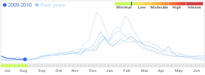
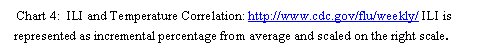
Observation of historical data indicates that flu related illnesses consistently start from November and last until May of each year. The following chart shows 2008 to 2009 flu trend in California.

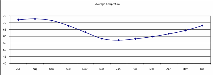
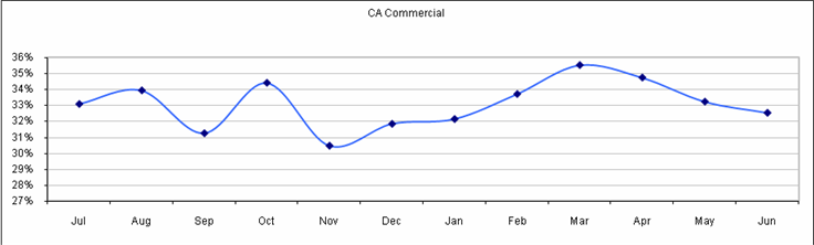
As you can see the flu season picks during the coldest months of the year, December to March. The following chart shows the daily average weather temperature trend in California for the same period of the time.

The table bellow shows the number of Health Net’s provider claim receipts for California commercial members and the number of California commercial members.

	Jul-08	Aug-08	Sep-08	Oct-08	Nov-08	Dec-08	Jan-08	Feb-08	Mar-08	Apr-08	May-08	Jun-08
Receipts	429,160	438,524	403,605	442,639	391,065	408,075	428,135	444,627	466,394	453,089	434,268	424,140
Membership	1,296,915	1,292,110	1,290,667	1,286,349	1,282,481	1,281,007	1,331,490	1,318,908	1,313,263	1,304,342	1,306,500	1,303,301
Receipts per Member	33.09%	33.94%	31.27%	34.41%	30.49%	31.86%	32.15%	33.71%	35.51%	34.74%	33.24%	32.54%

This analysis indicates that the number of receipts per member picks not in January-February, the coldest months of the year with the most flu related illnesses but in March. This perfectly correlates to the assumption of increased operating costs for managed health care companies during flu season. There is a lag time between a doctor visit and a claim submitted to the health insurance company by a provider. This lag time averages at a little above one month.

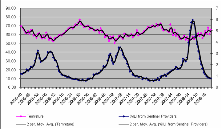
Influenza Like Illnesses (ILI) and Temperature Correlation

The regression analysis of ILI as a function of temperature indicates R=0.69 and R²=0.48. Low R² is explained by two factors: the ILI information presented by Center for Disease Control and Prevention (CDC) is presented in weekly break downs while the temperature information is in daily format. There is a margin of error in converting daily temperature to weekly format to be compared with ILI trend. Another factor is that individual observation points are not necessarily moving in opposite directions. However, the correlation between Temperature and ILI trend lines would hold significantly higher R².

Text Box: Chart 4: ILI and Temperature Correlation: http://www.cdc.gov/flu/weekly/ ILI is represented as incremental percentage from average and scaled on the right scale.

SUMMARY OUTPUT
Regression Statistics
Multiple R	0.6960837
R Square	0.4845325
Adjusted R Square	0.4807142
Standard Error	0.7963725
Observations	137
ANOVA
	df	SS	MS	F	Significance F
Regression	1	80.479981	80.479981	126.89817	3.661E-21
Residual	135	85.618237	0.6342092
Total	136	166.09822

	Coefficients	Standard Error	t Stat	P-value	Lower 95%	Upper 95%	Lower 95.0%	Upper 95.0%
Intercept	10.434298	0.7731665	13.495539	8.282E-27	8.9052135	11.963383	8.9052135	11.963383
	-0.1398187	0.0124119	-11.264909	3.661E-21	-0.1643656	-0.1152718	-0.1643656	-0.1152718

HDD

Weather Futures are traded in Chicago Mercantile Exchange (CME). The contracts are on the daily cumulative Heating Degree Days (HDD) and Cooling Degree Days (CDD) for a month observed at a weather station.

HDD=max (0,65-A) and CDD=max (0,A-65)

Where: A is the average of daily minimum and maximum temperatures. One Future contract is on $100 times the cumulative HDD or CDD for one full month. The historical temperature average provided in the Table 2 is measured in Los Angeles Civic Center. Historical trend is a reliable forecast for the future years since Weather Future Contracts have no systematic risk. This can be further adjusted for global warming effect.

1906-2008 averages in Los Angeles	Jul	Aug	Sep	Oct	Nov	Dec	Jan	Feb	Mar	Apr	May	Jun
Average Max	81.94	82.55	81.33	77.23	72.87	67.29	66.03	66.93	68.52	70.57	72.65	76.63
Average Min	62.55	63.19	61.90	58.35	53.30	49.23	48.19	49.38	51.03	53.13	55.97	59.20
Average Temperature	72.24	72.87	71.62	67.79	63.08	58.26	57.11	58.16	59.77	61.85	64.31	67.92
HDD	0.40	0.00	2.90	34.00	108.80	226.30	259.60	216.90	188.90	132.00	75.30	19.00
CDD	217.60	239.60	195.40	110.90	44.70	11.10	8.40	11.40	18.90	30.60	46.50	98.50

For Example, if we purchased one HDD future contract for January at a strike price of 200 and if the average temperature held our pay off would have been (259.60-200)*$100=$5,960.

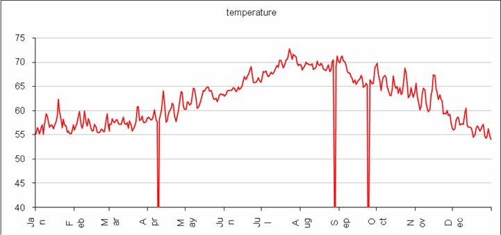
Historical average of daily HDD ranges from 0 to 9 and for month 0 to 270. However, HDD can reach as high as 750 in coldest parts of the world. Bellow is the temperature chart and a chart of deviation of my HDD calculation and WRCC HDD calculation based on historical daily average temperatures from1906 to 2008.

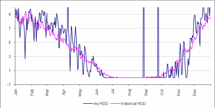
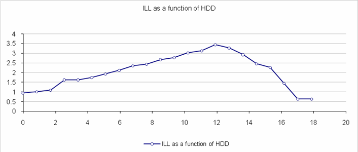
ILI as a Function of Temperature

Incremental percentage of ILI as a function of temperature is at its pick of 3.4% when the average of daily min and max temperature is 52 degrees of Fahrenheit. The drop in bellow 52 F is dictated by lack of data.

Text Box: Chart 7: incremental ILI as a Function of Temperature: http://www.cdc.gov/flu/weekly/
ILI is represented as incremental percentage from average

Similarly ILI incremental as a function of HDD is mirrored image of ILI as a function of temperature. As shown in Charts 5 and 6, HDD increases as the temperature decreases [HDD= max (0,65-A)].

Text Box: Chart 8: incremental ILI as a Function of HDD: http://www.cdc.gov/flu/weekly/
ILI is represented as incremental percentage from average

Scaling Expenses to HDD

The purpose of the project is to hedge the flu season ILI related claim expenses using HDD Weather Futures. Since our goal is to calculate the most optimal amount of extra expense to be hedged considering the cost of the future contracts, we need to convert HDD metrics into Dollar scale to be able to design the optimal cost-benefit probability model. Due to confidentiality of claim expense information I will use nominal values as Health Net’s ILI related claim costs. Please note that claim expense information is available for each month with doctor visit reason, visit date and claim date details. Let's assume that the extra claim expense during flu season has $12 mil historical mean (µ) and $3.2 mil standard deviation (σ). The historical HDD µ during Januaries is 260 with σ = 60. Therefore, $12 mil corresponds to 260 HDD and one degree of HDD corresponds to $3.2 mil/60= $53,333. Now to cover any expense over $12 mil extra expense, the 13th million and above for example, we will need to purchase one HDD at strike price 260 in our terms, which corresponds to $53,333/$100=533 HDD's, again, at 260 strike price. Going forward we will discuss the project in dollar terms, which can be converted into real HDD terms using the scale matching strategy in this section.

Cost of Debt

Our objective is to find futures' optimal strike price and volume to hedge the enterprise expenses against volatility. For this purpose we introduce the volatility cost of enterprise. On the other hand we shall introduce the profit margin of the issuer of futures. In our model the average amount of ILI related expenses (µ) is equal to $12 mil and the variance (σ) is equal to $3.2 mil. The cost of the volatility is introduced via two parameters. A debt cost (debtc) in the case when the enterprise expenses end up at their mean (µ), and a multiplication factor (debtk) by which the debt cost of enterprise would increase if the company ends up with an expense higher from the average by σ (i.e. µ + σ). The higher is debtk the higher is the interest to stay closer to µ (the average being equal to µ).

We assume that the default debt cost (debtc) is equal to $300’000 (the default price applicable for all scenarios where expenses end up at the average of $12 mil). The multiplication factor (debtk) is a parameter changing from 1.5 to 5. For instance if this factor is 2, it means that if the enterprise ends up with an expense of $15.2 mil (i.e. one σ away from the µ), it will cost extra $600’000 to the company (e.g. due to short-term debt interests).

Price probability density transformation

In this section we analyze transformations of a probability density of an operation cost, caused by purchases of futures (issued on the same level of the cost). We assume two free variables in the purchasing of futures, the strike price and the quantity of futures. We assume that all futures are purchased with the same strike price. When the operation cost exceeds the strike price, the futures cover the given percentage of the operation cost excess. That percentage depends on the amount of futures purchased. It can vary from 0% to 100% (underinsurance) or can be more than 100% (over-insurance). The choice of the quantity of purchased futures determines the insurance ratio.

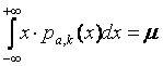
The probability density of the hedged price is computed as follows:

Where:

c is the cost of purchased futures

a is the strike price

k is the insurance ratio (1 corresponds to 100%)

Obviously:

The following animation shows how the probability curve of price changes when the ratio of insurance changes from 10% to 250%. The strike price is the same in all samples. The cost of futures is computed with a very simplified empiric formula (it is sufficient for this demonstration). As expected, this animation shows that the more you increase the insurance ratio toward 100%, the narrower the volatility of your prices becomes. We also see that the price, when over insured, never exceeds the strike price plus the cost of insurance.

Animation link:

http://switzernet.com/people/aram-gabrielyan/public/090817-hedging-cost-with-futures/

Neutral (right) price of Futures

Let us have an operation price probability, a subject to normal Gaussian distribution (see normal distribution):

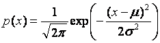
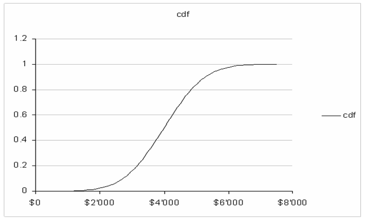
The following chart shows such distribution, where the mean value is equal to $4’000 and the variance is equal to $1’000:

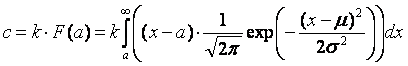
We seek to compute the ‘right’ price of futures (issued for our operation cost) as a function of the strike price a. Such futures pay-off each additional $1 of operation cost exceeding the selected strike price a.

The statistical ‘margin-less’ cost of such futures must be equal to:

The cost computed in such a way contains neither a security nor a beneficiary margin of the issuer of futures.

Using the above formula the joined Excel file computes the cost of futures straight-forwardly by summing refund claims weighted by their probabilities. For each price exceeding the strike price, the formula takes the difference between the price and the strike-price, multiplies it by the probability of the price, and adds all of them together. The final sum is multiplied by the distance between the sample points on the x axis.

Our objective is to find the analytical formula of the price of futures (and if not analytical then one using well known functions, such as the error function).

Due to the symmetric bell shape of the normal distribution:

Therefore:

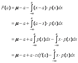
CDF is the cumulative distribution function [see normal distribution]. It represents the probability that the price will fall below x (its argument).

[xls]

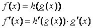
Considering the product rule (see derivative):

We can write that:

Therefore:

CDF can be expressed via error function as follows (see normal distribution):

ERF Excel function is implemented so no approximations or simulations is needed.

It is known that (see list of integrals):

Taking into account the chain rule (see derivative):

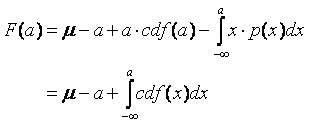
The CDF integral is computed as follows:

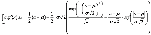
The ‘margin-less’ price of futures can be therefore expressed as follows:

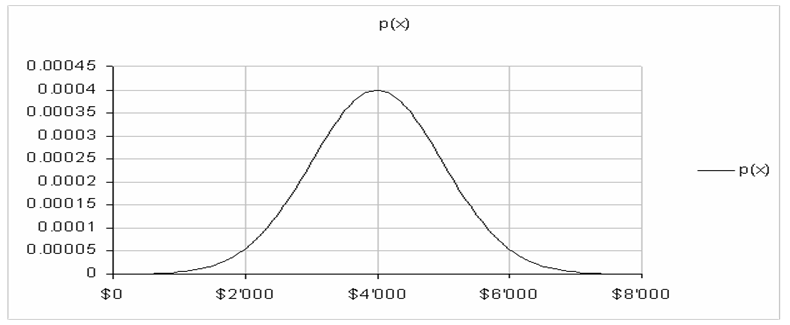
The following animation shows the price of futures as a function of the strike price where the variance, i.e. the volatility, changes from $100 to $6500 over the time. The mean value is always the same and is equal to $4000:

Animation link:

http://switzernet.com/people/aram-gabrielyan/public/090819-neutral-price-vs-Black-Scholes/

Probability density function of insured costs and futures with right prices

In Price probability density transformation [090817 ii] we developed the probability density function of operation costs insured by futures. This density is also a function of selected strike price and of insurance ratio k (representing the pay-off ratio of cost units exceeding the strike price a, or otherwise the amount of purchased futures). In the document we assumed the cost of futures c as an input parameter. No formula was provided for computing the cost of futures.

In Neutral (right) price of Futures [090819 ii] we developed a formula for computing the ‘right’ cost of futures for a given strike price a. Under term ‘right’ or ‘neutral’ we understand the price, such futures would cost to an insurance company taking into account the volatility of the cost. This shall be an integral of excess of operation prices exceeding the strike price a weighted by the normal distribution of the operation price (see normal distribution).

The formula of futures price that we developed in [090819 ii], is fully analytical, with the exception of error function ERF implemented in Excel (see error function).

Because the price of futures is right, if computed as follows:

The following must hold for all a and k

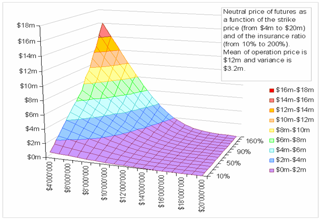
In order to validate both of our formulas, we use an Excel model. The mean of our operation cost at $12 mil and the variance is $3.2 mil. For a two-dimensional set of parameters, (a) strike prices varying from $4 mil to $20 mil and (b) the insurance ratios varying from 10% to 200%, we compute ‘right’ prices of futures using our formula . The blow chart shows this function for the two dimensional set of input parameters:

Sub-sequentially, based on the right price, we compute probability density values with our formula by loading results into an array with prices ranging from $0 to $23’500’000.

The following animation shows that the choice of a and k can change the shape of price distribution significantly:

Animation link:

http://switzernet.com/people/aram-gabrielyan/public/090819-average-of-hedged-cost/

By having, for each shape (dictated by a pair of strike price a and insurance ratio k) of the probability density array we compute the mean of the insured operation cost:

Irrespectively how wildly the probability density shape is changed (by the choice of two parameters of futures), the Excel simulation shows that the computed mean of insured operation costs is always equal to the mean of the uninsured costs, i.e. to µ (with exceptions of precision errors). This suggests no hidden costs in prices of futures.

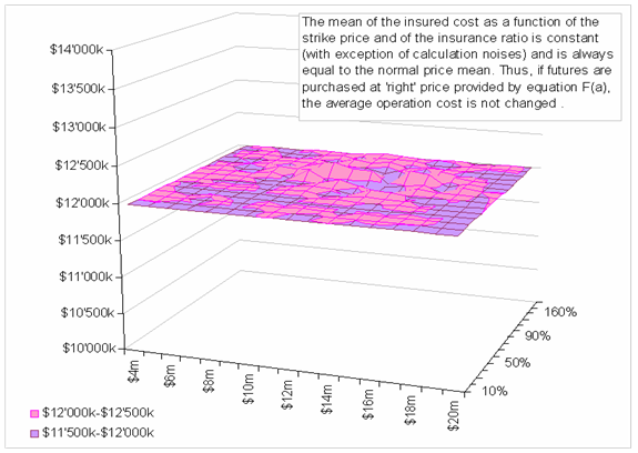
The results of this simulation validate our two formulas for calculation of the ‘right’ price of futures and subsequent calculation of the insured costs' probability density .

Finding the optimal strike price and volume of futures

In our model we deal with future contracts that can pay-off a portion of enterprise expenses exceeding a pre-selected strike price. The choice of the pay-off portion (of the excess with respect to the strike price) is made by the choice of the amount of purchased futures. This fraction can be less than, more than, or equal to 1. This model is applicable to a more general case, where instead of futures issued directly on the enterprise expenses, the futures are issued on another underlying instrument highly correlated to the enterprise expenses. HDD future contracts are a good example of such instruments.

Our objective is to find the optimal strike price and volume of futures, purchased for hedging the enterprise expenses against volatility (see Cost of Debt section.)

In [090817 ii] we developed price probability density transformation achieved by the purchase of futures. In [090819a ii] we developed a formula for computing the neutrally or right price of futures. In [090819b ii] we showed that the mean of insured expenses does not change, if the futures are bought at neutrally right prices. This means that if the market price of futures is always right, we are definitely interested in purchasing futures all the time, even if the volatility cost is low. Futures are narrowing the probability density of expenses and are therefore minimizing the volatility related debt costs.

However the pleasure of having a future based insurance shall often have a market cost exceeding its neutrally right price [090819a ii]. The difference between the market price of futures and the right price computed by our formulas [090819a ii] is precisely the cost of this pleasure. This cost must be counterbalanced with savings achieved on the volatility side. The margin added on the right price of futures is represented in percentages. We analyze a range from 0.5% to 90%.

In the following chart we assume that the default debt cost (debtc) is equal to $300’000 (the default price applicable for all scenarios where expenses end up at the average of $12 mil). The multiplication factor (debtk) is a parameter changing from 1.5 to 5. For instance if this factor is 2, it means that if the enterprise ends up with an expense of $15.2 mil (i.e. one variance away from the mean), it will cost extra $600’000 to the company (e.g. due to short-term debt interests) (see Cost of Debt section.)

The surface shown in the animation below represents the overall cost (the volatility debt cost together with the profit margins paid to issuers of futures) as a function of the strike price (in the range from $4 mil to $20 mil) and the insurance ratio (in the range from 10% to 200%). The animation shows the changes in the shape when changing the issuer's profit margin (fairness) and the debt cost factor (dependence). For each frame (i.e. for each pair of fairness of futures and dependence of enterprise from the volatility), the text data panel shows the best recommended strike price and insurance ratio.

This animation demonstrates the concave shaped form of the surface for all pairs of fairness and dependence showing that there is always an optimal choice to make depending on the market prices of futures and the extra cost of the volatility of the enterprise expenses.

Animation link:

http://switzernet.com/people/aram-gabrielyan/public/090820-best-strike/