The basics of line moiré patterns and optical speedup
Emin Gabrielyan
emin.gabrielyan@switzernet.com
2007-03-02
1. Table of contents
The basics of
line moiré patterns and optical speedup
4.1...... Superposition of layers with periodically repeating
parallel lines
4.2...... Speedup of movements with moiré
4.3...... Superposition of layers with inclined lines
4.3.1. Computing moiré lines’ inclination as function of the
inclination of layers’ lines
4.3.2. Deducing the known formulas from our equations
4.3.3. The revealing lines inclination as a function of the
superposition image’s lines inclination
5. Superposition of periodic circular patterns
5.1...... Superposition of circular periodic patterns with
radial lines
5.2...... Superposition of circular patterns with radial curves
2. Abstract
We are addressing the optical speedup of movements of layers in moiré
patterns. We introduce a set of equations for computing curved patterns, where
the formulas of optical speedup and moiré periods are kept in their simplest
form. We consider linear movements and rotations. In the presented notation,
all periods are relative to the axis of movements of layers and moiré bands.
3. Introduction
Moiré patterns appear when
superposing two transparent layers containing correlated opaque patterns. The
case when layer patterns comprise straight or curved lines is called line
moiré.
This document presents the
basics of line moiré patterns. We present numerous examples and we focus also on
the optical speedup of moiré shapes when moving layer patterns. Numerous
examples are present. Dynamic examples demonstrating the movements of layers
are presented by GIF files.
We develop here the most
important formulas for computing the periods of superposition patterns, the
inclination angles and the velocities of optical shapes when moving one of the
layers.
In section 4, we demonstrate the phenomenon on the examples with
horizontal parallel lines, which are further extended to cases with inclined
and curved lines. In section 5 we present circular examples with straight radial
lines, which are analogously extended.
4. Simple moiré patterns
4.1. Superposition of layers with periodically repeating parallel lines
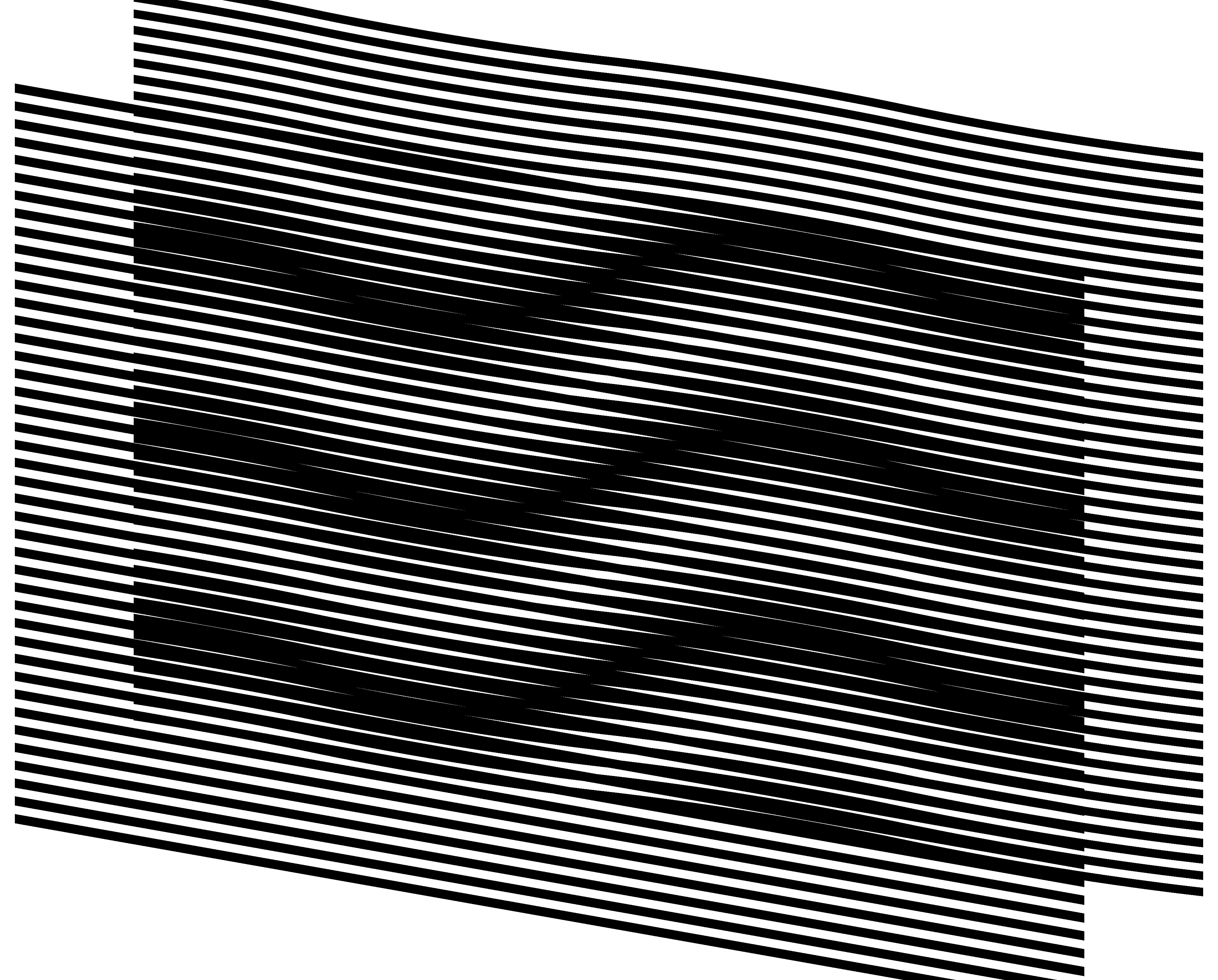
Simple moiré patterns can be observed when superposing two transparent layers comprising periodically repeating opaque parallel lines as shown in Figure 1. The lines of one layer are parallel to the lines of the second layer.
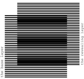
Figure 1. Superposition of two layers consisting of parallel lines, where the lines of the revealing layer are parallel to the lines of the base layer [eps], [tif], [png]
The superposition image does not change if transparent
layers with their opaque patterns are inverted. We denote one of the layers as
the base layer and the other one as
the revealing layer. When considering
printed samples, we assume that the revealing layer is printed on a
transparency and is superposed on top of the base layer, which can be printed either
on a transparency or on an opaque paper. The periods of the two layer patterns,
i.e. the space between the axes of parallel lines, are close. We denote the
period of the base layer as ![]() and the period of the
revealing layer as
and the period of the
revealing layer as ![]() . In Figure
1, the period of lines of the base layer is equal to 6
units, and the period of lines of the revealing layer is equal to 5.5 units.
. In Figure
1, the period of lines of the base layer is equal to 6
units, and the period of lines of the revealing layer is equal to 5.5 units.
The superposition image of Figure 1 outlines periodically repeating dark parallel bands, called moiré lines. Spacing between the moiré lines is much larger than the periodicity of lines in the layers.
Light areas of the superposition image correspond to the zones where the lines of both layers overlap. The dark areas of the superposition image forming the moiré lines correspond to the zones where the lines of the two layers interleave, hiding the white background. The labels of Figure 2 show the passages from light zones with overlapping layer lines to dark zones with interleaving layer lines. The light and dark zones are periodically interchanging.
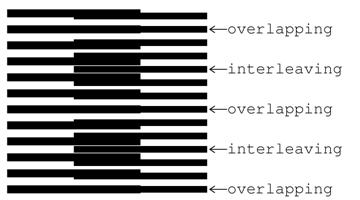
Figure 2. Superposition of two layers consisting of horizontal parallel lines [eps], [tif], [png]
Figure 3 shows a detailed diagram of the superposition image between two light zones, where the lines of the revealing and base layers overlap [Sciammarella62a, p. 584].
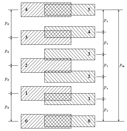

Figure 3. Computing the period of moiré lines in a superposition image as a function of the periods of lines of the revealing and base layers
The period ![]() of moiré lines is the
distance from one point where the lines of both layers overlap (at the bottom
of the figure) to the next such point (at the top). Let us count the layer lines,
starting from the point where they overlap. Since in our case
of moiré lines is the
distance from one point where the lines of both layers overlap (at the bottom
of the figure) to the next such point (at the top). Let us count the layer lines,
starting from the point where they overlap. Since in our case ![]() , for the same number of counted lines, the base layer lines with
a long period advance faster than the revealing layer lines with a short period.
At the halfway of the distance
, for the same number of counted lines, the base layer lines with
a long period advance faster than the revealing layer lines with a short period.
At the halfway of the distance ![]() , the base layer lines are ahead the revealing layer lines by
a half a period (
, the base layer lines are ahead the revealing layer lines by
a half a period (![]() ) of the revealing layer lines, due to which the lines are
interleaving, forming a dark zone. At the full distance
) of the revealing layer lines, due to which the lines are
interleaving, forming a dark zone. At the full distance ![]() , the base layer lines are ahead of the revealing layer lines
by a full period
, the base layer lines are ahead of the revealing layer lines
by a full period ![]() , so the lines of the layers again overlap. The base layer
lines gain the distance
, so the lines of the layers again overlap. The base layer
lines gain the distance ![]() with as many lines (
with as many lines (![]() ) as the number of the revealing layer lines (
) as the number of the revealing layer lines (![]() ) for the same distance minus one:
) for the same distance minus one:
From equation (4.1) we obtain the well known formula for the period ![]() of the superposition image
[Amidror00a, p.20]:
of the superposition image
[Amidror00a, p.20]:
The superposition of two layers comprising parallel lines forms an optical image comprising parallel moiré lines with a magnified period. According to equation (4.2), the closer the periods of the two layers, the stronger the magnification factor is.
If the numbers ![]() and
and ![]() are
integers, then if at some moiré light zone the lines of both layers perfectly
overlap, as shown in Figure
3, the layer lines will also perfectly overlap also at
the centers of each other light zone. If
are
integers, then if at some moiré light zone the lines of both layers perfectly
overlap, as shown in Figure
3, the layer lines will also perfectly overlap also at
the centers of each other light zone. If ![]() and
and ![]() are not integers, then
the centers of white moiré zones do not necessarily match with the centers of
layer lines. In any case, equation (4.2) remains valid.
are not integers, then
the centers of white moiré zones do not necessarily match with the centers of
layer lines. In any case, equation (4.2) remains valid.
For the case when the revealing layer period is longer than the base layer period, the space between moiré lines of the superposition pattern is the absolute value of formula of (4.2).
The thicknesses of layer lines affect the
overall darkness of the superposition image and the thickness of the moiré
lines, but the period ![]() does not depend on the
layer lines’ thickness. In our examples the base layer lines’ thickness is
equal to
does not depend on the
layer lines’ thickness. In our examples the base layer lines’ thickness is
equal to ![]() , and the revealing layer lines’ thickness is equal to
, and the revealing layer lines’ thickness is equal to ![]() .
.
4.2. Speedup of movements with moiré
The moiré bands of Figure 1 will move if we displace the revealing layer. When
the revealing layer moves perpendicularly to layer lines, the moiré bands move along
the same axis, but several times faster than the movement of the revealing layer.
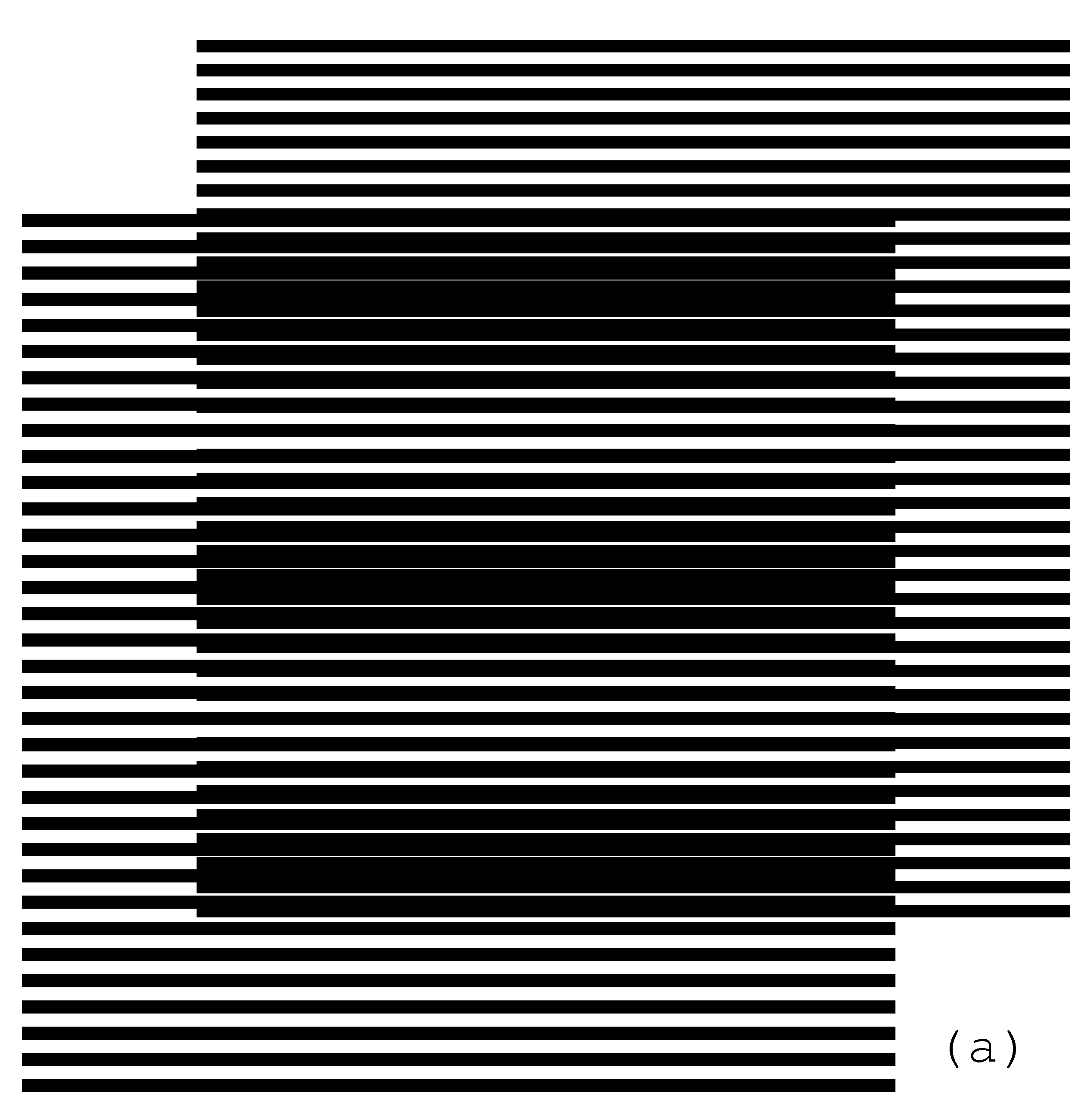
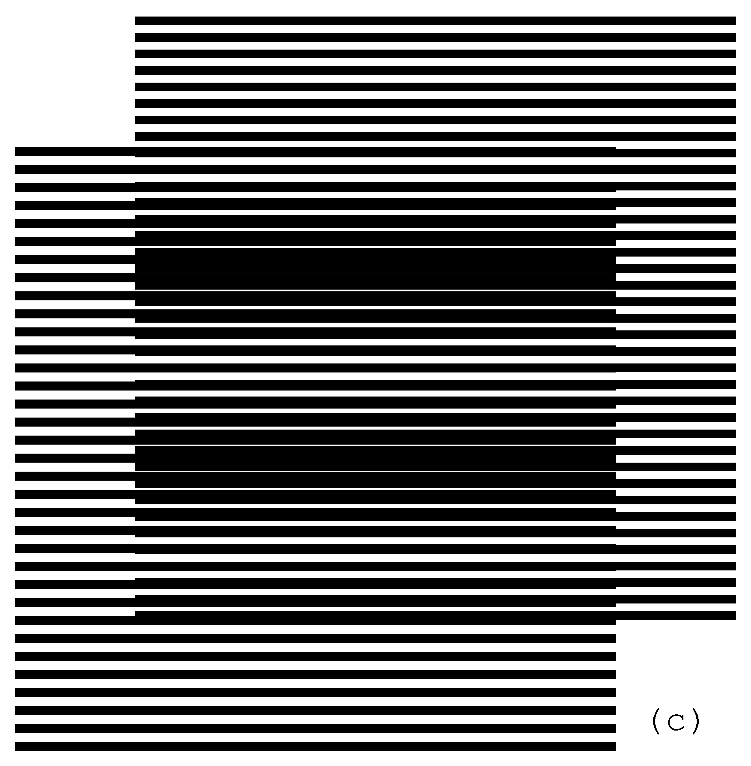
The three images of Figure
4 show the superposition image for different positions
of the revealing layer. In the second image (b) of Figure 4, compared to the first image (a), the revealing layer
is shifted up by one third of the revealing layer period (![]() ). In the third image (c), compared to the first image (a), the
revealing layer is shifted up by two third of the revealing layer period (
). In the third image (c), compared to the first image (a), the
revealing layer is shifted up by two third of the revealing layer period (![]() . The images show that the moiré lines of the superposition
image move up at a speed, much faster than the speed of movement of the
revealing layer.
. The images show that the moiré lines of the superposition
image move up at a speed, much faster than the speed of movement of the
revealing layer.
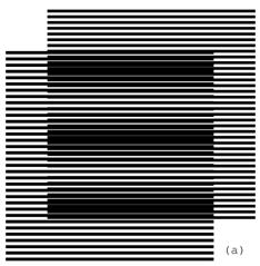
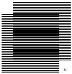
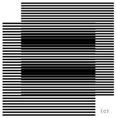
Figure 4. Superposition of two layers with parallel horizontal lines, where the revealing layer moves vertically at a slow speed [eps (a)], [png (a)], [eps (b) ], [png (b)], [eps (c)], [png (c)]
When the revealing layer is shifted up
perpendicularly to the layer lines by one full period ![]() of its pattern, the
superposition optical image must be the same as the initial one. It means that the
moiré lines traverse a distance equal to the period of the superposition image
of its pattern, the
superposition optical image must be the same as the initial one. It means that the
moiré lines traverse a distance equal to the period of the superposition image ![]() while the revealing
layer traverses the distance equal to its period
while the revealing
layer traverses the distance equal to its period ![]() . Assuming that the base layer is immobile (
. Assuming that the base layer is immobile (![]() ), the following equation holds for the ratio of the optical
image’s speed to the revealing layer’s speed:
), the following equation holds for the ratio of the optical
image’s speed to the revealing layer’s speed:
According to equation (4.2) we have:
In case the period of the revealing layer is longer than the period of the base layer, the optical image moves in the opposite direction. The negative value of the ratio computed according to equation (4.4) signifies the movement in the reverse direction.
The GIF animation of the superposition image corresponding
to a slow movement of the revealing layer is provided in Figure 5. The GIF file repeatedly animates a perpendicular movement
of the revealing layer across a distance equal to ![]() .
.
Figure 5. GIF animation of the slow vertical movement of the revealing layer [ps], [gif], [tif]
4.3. Superposition of layers with inclined lines
In this section we develop equations for
patterns with inclined lines. Since most of all we are interested in optical
speedup, instead of using the well known equations, we represent the case of inclined
patterns such that the equations (4.2), (4.3), and (4.4) remain valid in their current simple form. The values
of periods ![]() ,
, ![]() , and
, and ![]() for the examples of Figure 4 correspond to the distances between the lines along
the vertical axis corresponding to the axis of movements. When the layer lines
are horizontal (or perpendicular to the movement axis) the periods (p) are equal to the distances (denoted
as T) between the lines (as in Figure 1, Figure
3, and Figure
4). If the lines are inclined the periods (p) along the vertical axis does not
correspond anymore to the distances (T)
between the lines. According to our notations, the periods p do not represent the distances T between the lines, but the distances between the lines along the
axis of movements. By adopting the new notation, equations (4.2), (4.3), and (4.4) are valid all the time. Equations for inclination
angles for such notation of periods (p)
are presented in this section. For rotational movements p values represent the periods along circumference, i.e. the
angular periods.
for the examples of Figure 4 correspond to the distances between the lines along
the vertical axis corresponding to the axis of movements. When the layer lines
are horizontal (or perpendicular to the movement axis) the periods (p) are equal to the distances (denoted
as T) between the lines (as in Figure 1, Figure
3, and Figure
4). If the lines are inclined the periods (p) along the vertical axis does not
correspond anymore to the distances (T)
between the lines. According to our notations, the periods p do not represent the distances T between the lines, but the distances between the lines along the
axis of movements. By adopting the new notation, equations (4.2), (4.3), and (4.4) are valid all the time. Equations for inclination
angles for such notation of periods (p)
are presented in this section. For rotational movements p values represent the periods along circumference, i.e. the
angular periods.
4.3.1. Computing moiré lines’ inclination as function of the inclination of layers’ lines
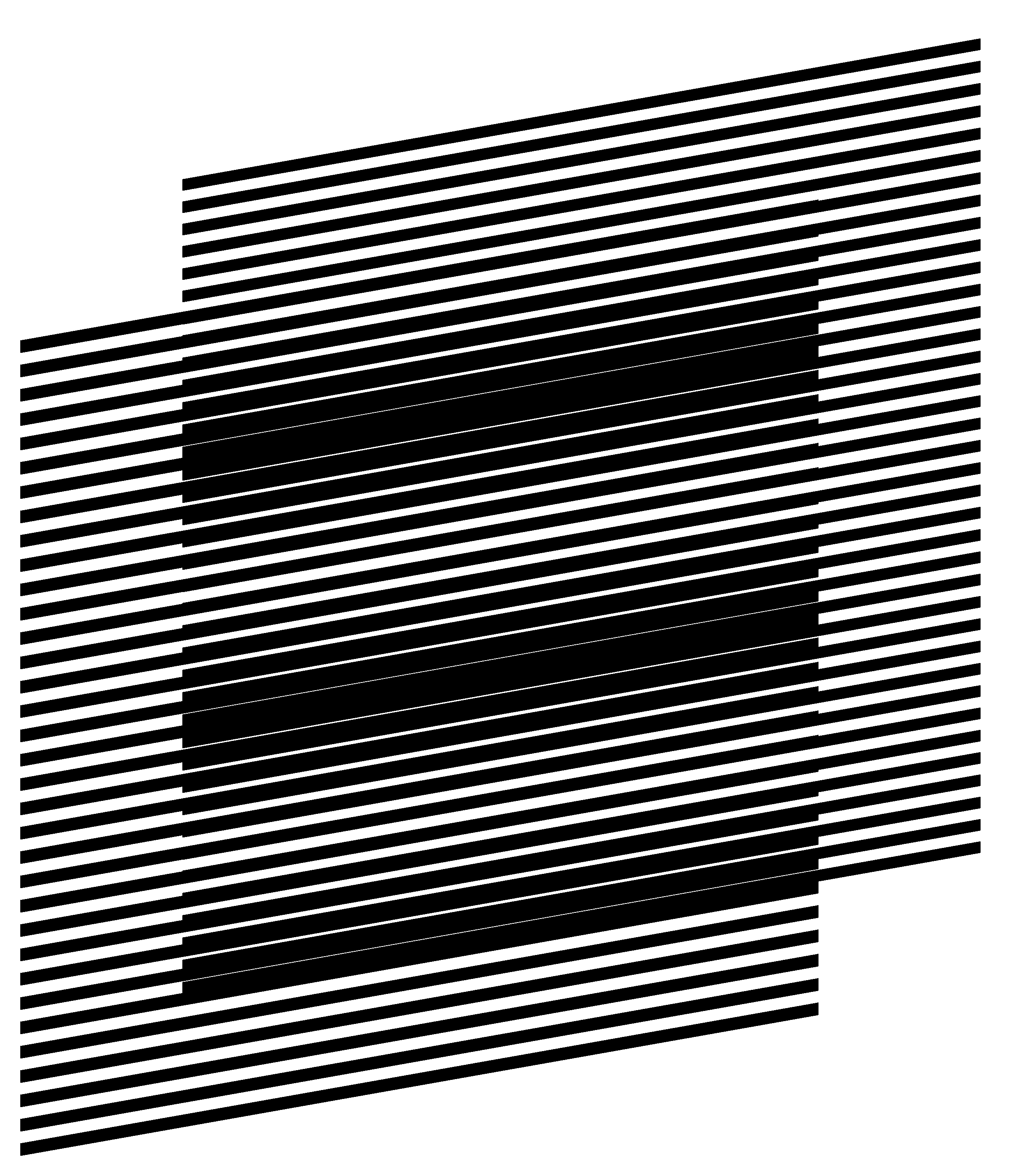
The superposition of two layers with identically
inclined lines forms moiré lines inclined at the same angle. Figure 6 is obtained from Figure
1 with a vertical shearing. In Figure 6 the layer lines and the moiré lines are inclined by
10 degrees. Inclination is not a rotation. During the inclination the distance
between the layer lines along the vertical axis (p) is conserved, but the true distance T between the lines (along an axis perpendicular to these lines)
changes. The diagram of Figure
10 shows the difference between the vertical periods ![]() and
and ![]() , and the distances
, and the distances ![]() and
and ![]() .
.
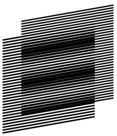
Figure 6. Superposition of layers consisting of inclined parallel lines where the lines of the base and revealing layers are inclined at the same angle [eps], [png]
The inclination degree of layer lines may change
along the horizontal axis forming curves. The superposition of two layers with
identical inclination pattern forms moiré curves with the same inclination
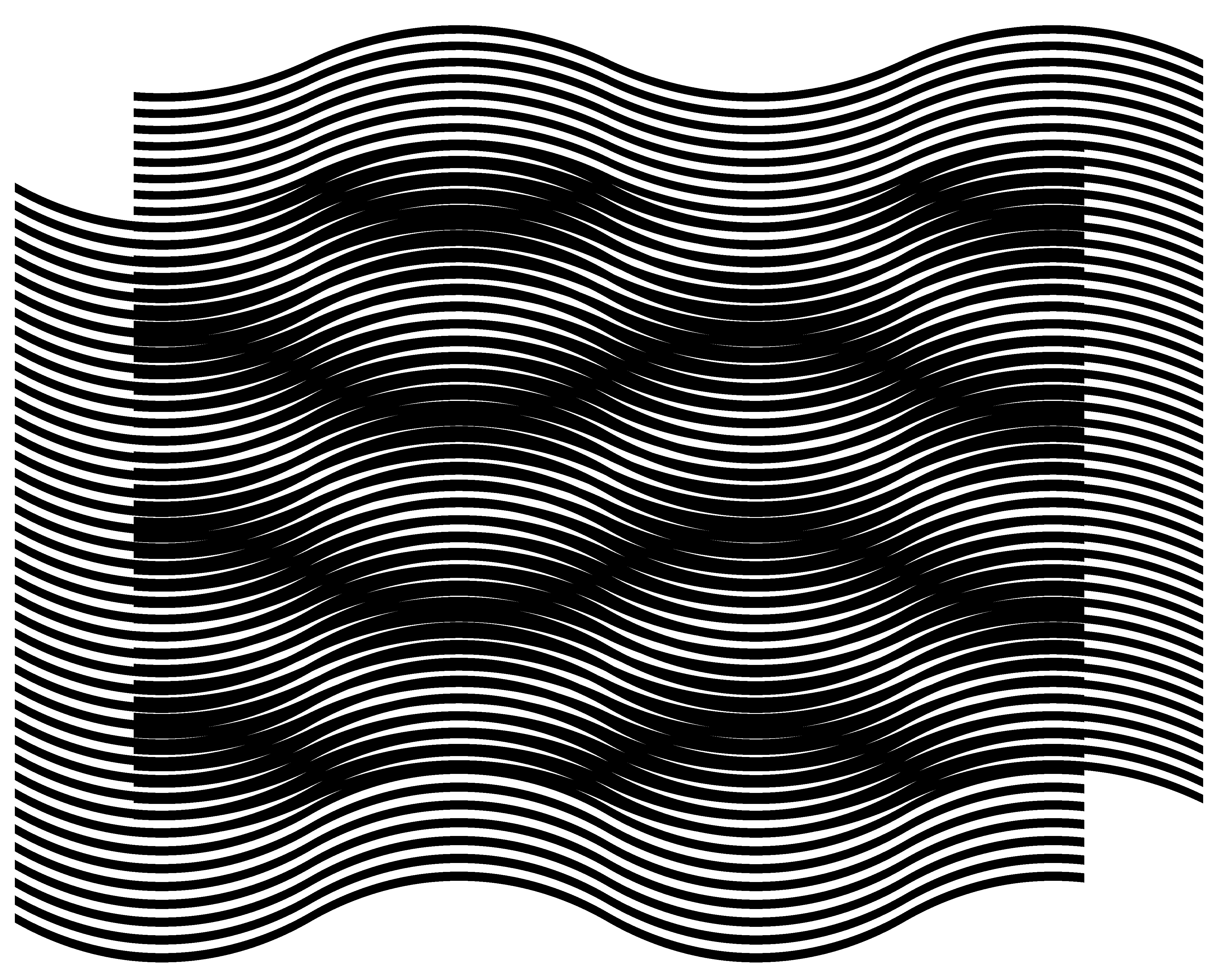
pattern. In Figure 7 the inclination degree of layer lines gradually
changes according the following sequence of degrees (+30, –30, +30, –30, +30),
meaning that the curve is divided along the horizontal axis into four equal
intervals and in each such interval the curve’s inclination degree linearly
changes from one degree to the next according to the sequence of five degrees. Layer
periods ![]() and
and ![]() represent the distances
between the curves along the vertical axis. In Figure 6 and Figure
7,
represent the distances
between the curves along the vertical axis. In Figure 6 and Figure
7, ![]() is equal to 6 units
and
is equal to 6 units
and ![]() is 5.5. units. Figure 7 can be obtained from Figure 1 by interpolating the image along the horizontal axis
into vertical bands and by applying a corresponding vertical shearing and
shifting to each of these bands. Equation (4.2) is valid for computing the spacing
is 5.5. units. Figure 7 can be obtained from Figure 1 by interpolating the image along the horizontal axis
into vertical bands and by applying a corresponding vertical shearing and
shifting to each of these bands. Equation (4.2) is valid for computing the spacing ![]() between the moiré
curves along the vertical axis and equation (4.4) for computing the optical speedup ratio when the
revealing layer moves along the vertical axis.
between the moiré
curves along the vertical axis and equation (4.4) for computing the optical speedup ratio when the
revealing layer moves along the vertical axis.
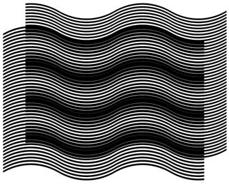
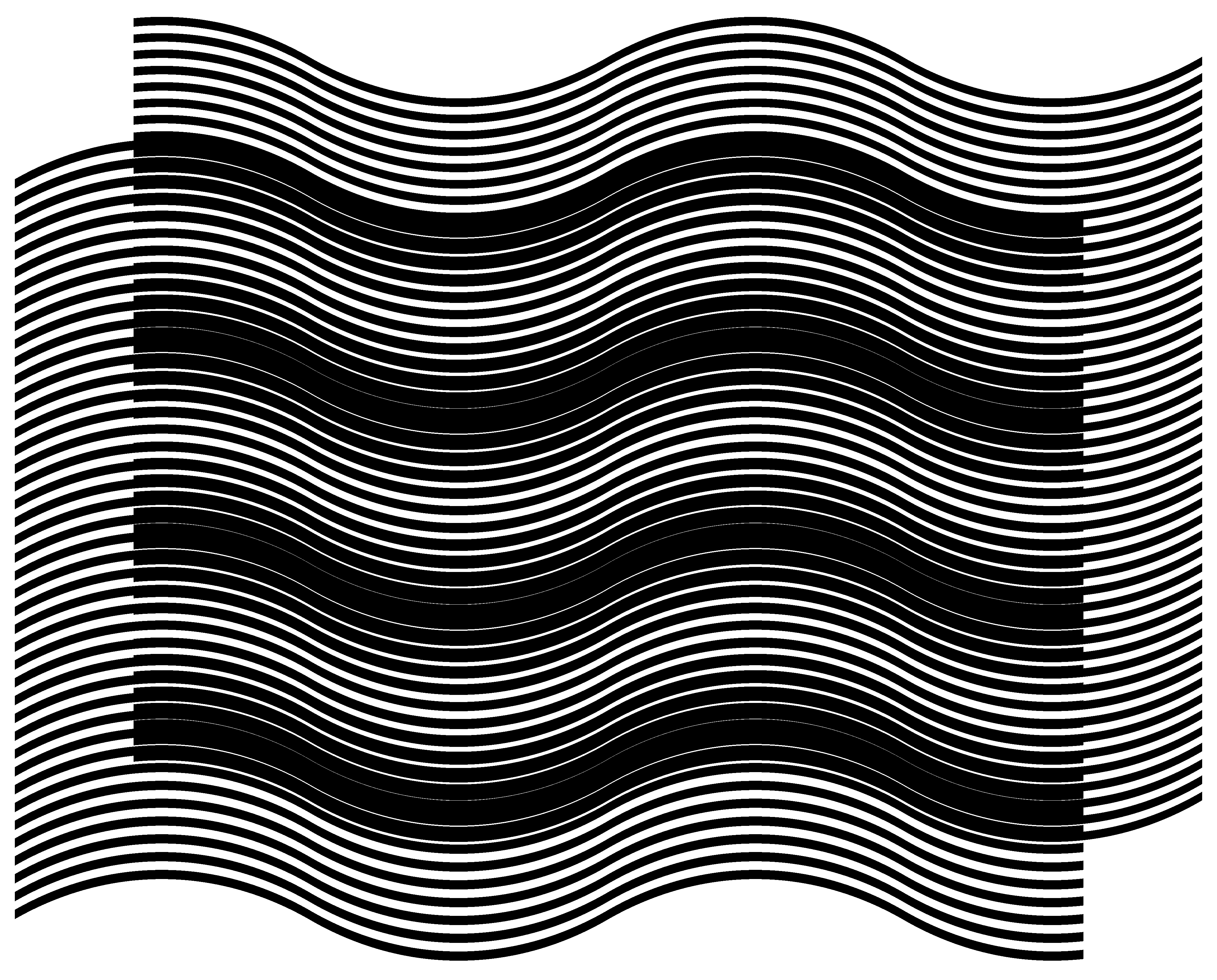
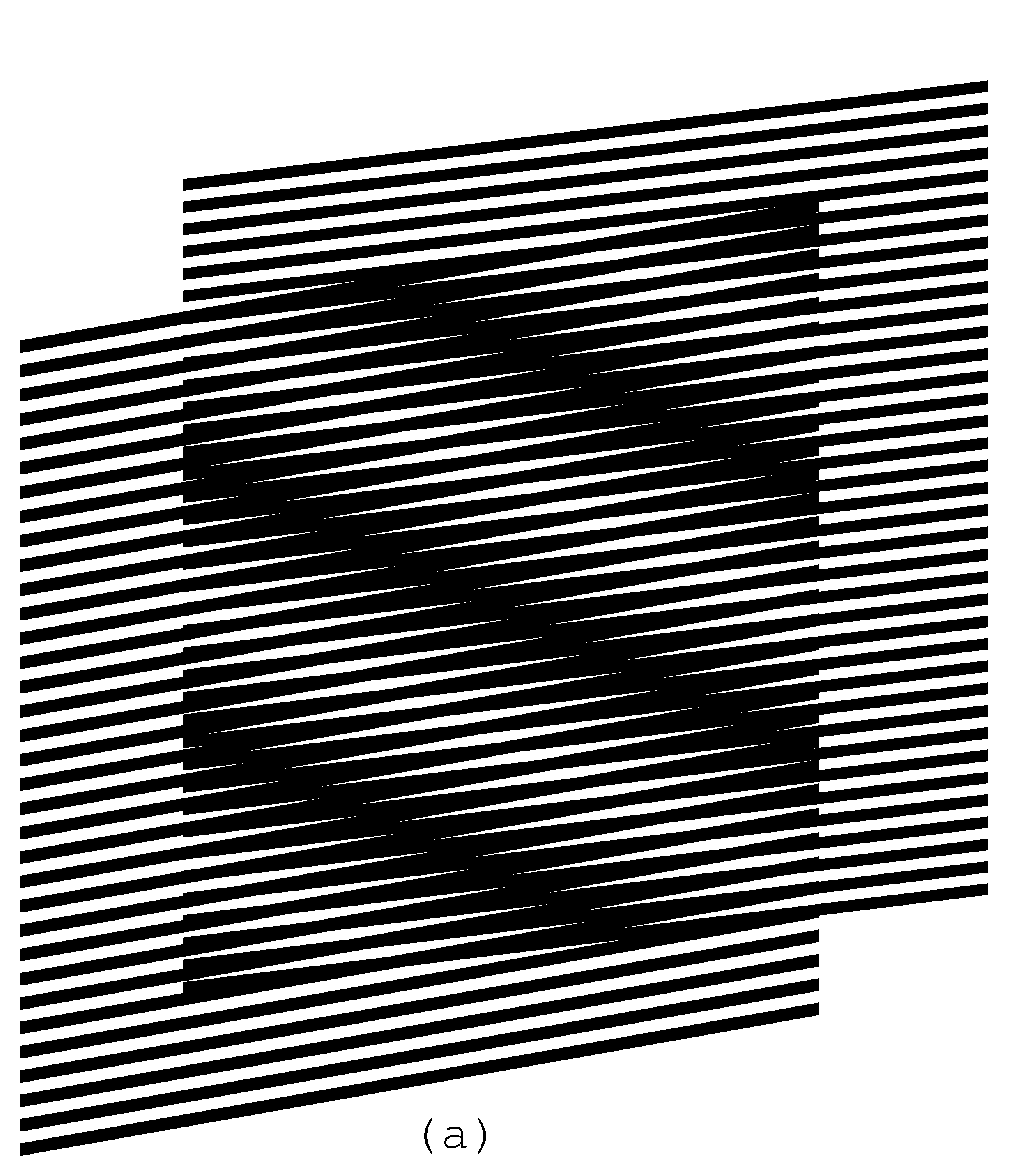
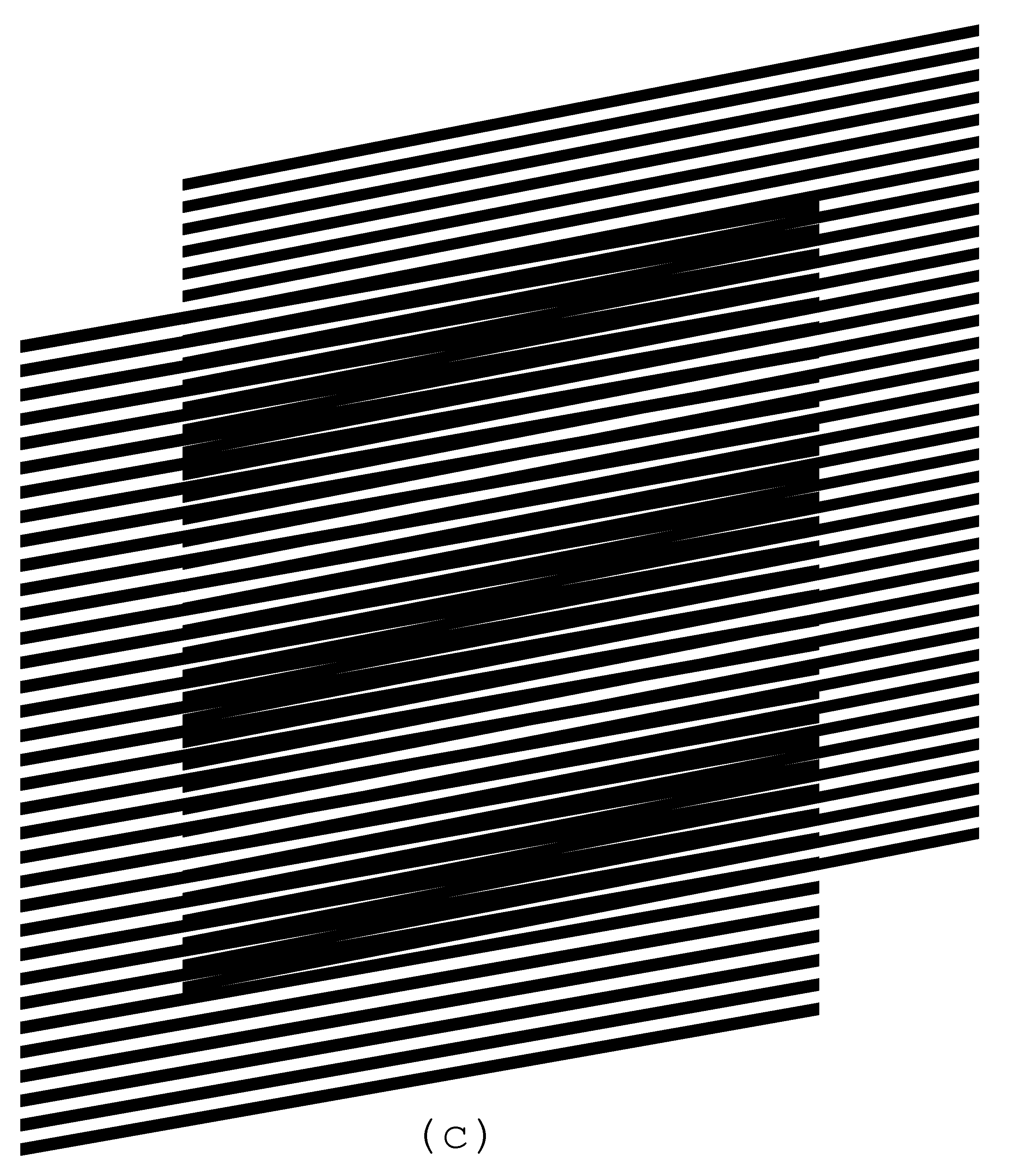
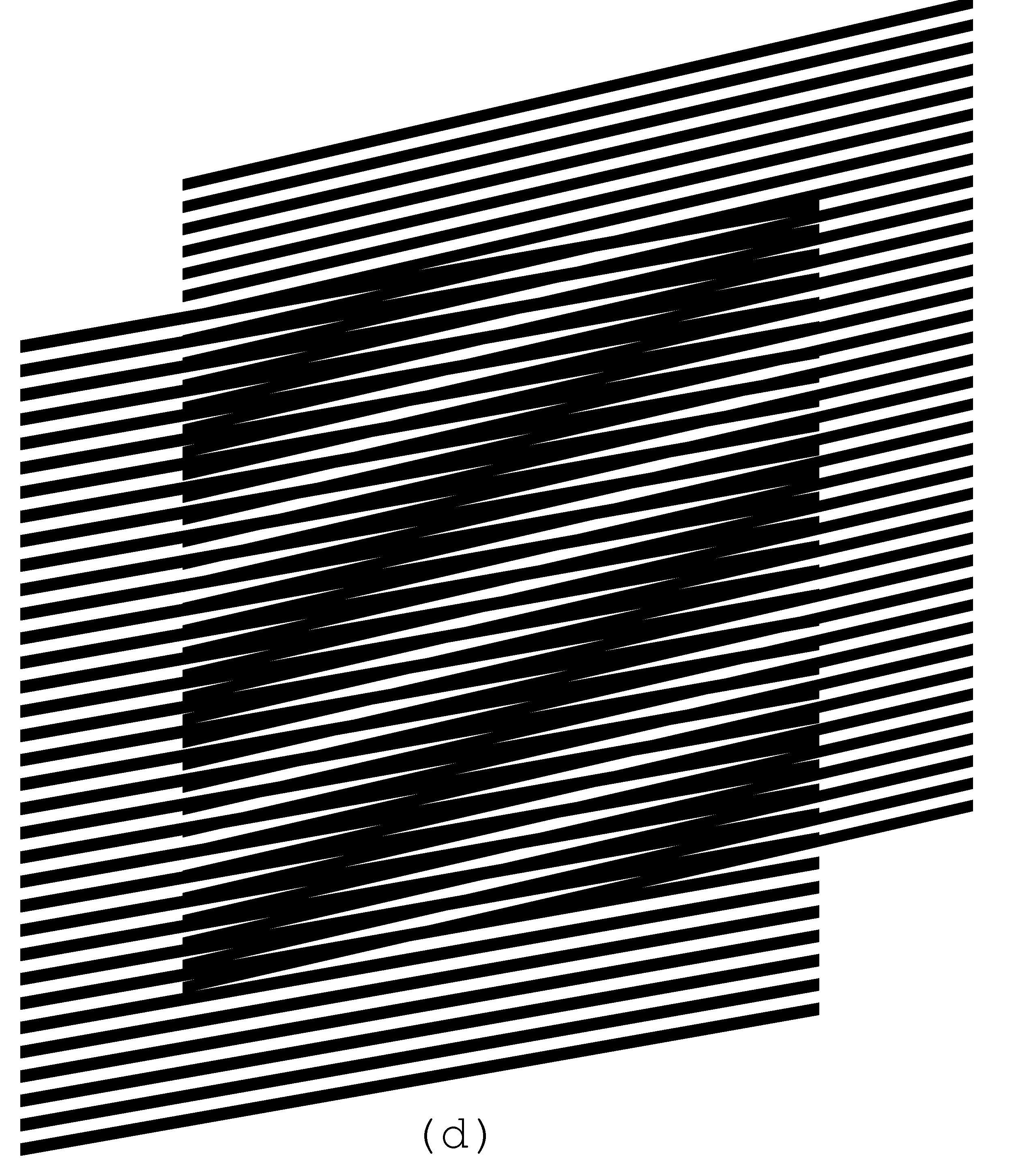
Figure 7. Two layers consisting of curves with identical inclination patterns, and the superposition image of these layers [eps], [png]
More interesting is the
case when the inclination degrees of layer lines are not the same for the base
and revealing layers. Figure
8 shows four superposition images where the inclination
degree of base layer lines is the same for all images (10 degrees), but the inclination
of the revealing layer lines is different for images (a), (b), (c), and (d) and
is equal to 7, 9, 11, and 13 degrees correspondingly. The periods of layers
along the vertical axis ![]() and
and ![]() (6 and 5.5 units
correspondingly) are the same for all images. Correspondingly, the period
(6 and 5.5 units
correspondingly) are the same for all images. Correspondingly, the period ![]() computed with equation
(4.2) is also the same for all images.
computed with equation
(4.2) is also the same for all images.
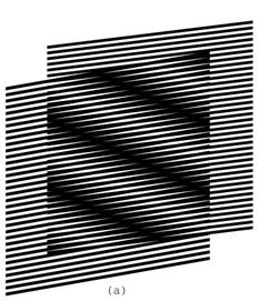
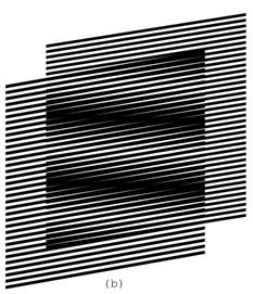
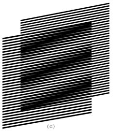
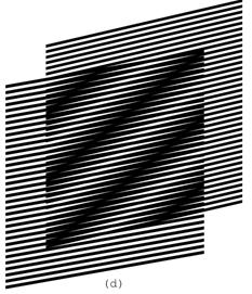
Figure 8. Superposition of layers consisting of inclined parallel lines, where the base layer lines’ inclination is 10 degrees and the revealing layer lines’ inclination is 7, 9, 11, and 13 degrees [eps (a)], [png (a)], [eps (b)], [png (b)], [eps (c)], [png (c)], [eps (d)], [png (d)]
The GIF animation of Figure 9 shows the superposition image when the revealing layer’s inclination oscillates between 5 and 15 degrees:
Figure 9. GIF animation, where the inclination of parallel lines of the revealing layer oscillates between 5 and 15 degrees [ps], [gif], [tif]
Figure
10 helps to compute the inclination degree of moiré optical
lines as a function of the inclination of the revealing and the base layer
lines. We draw the layer lines schematically without showing their true
thicknesses. The bold lines of the diagram inclined by ![]() degrees are the base
layer lines. The bold lines inclined by
degrees are the base
layer lines. The bold lines inclined by ![]() degrees are the
revealing layer lines. The base layer lines are vertically spaced by a distance
equal to
degrees are the
revealing layer lines. The base layer lines are vertically spaced by a distance
equal to ![]() , and the revealing layer lines are vertically spaced by a
distance equal to
, and the revealing layer lines are vertically spaced by a
distance equal to ![]() . The distances
. The distances ![]() between the base layer
lines and the distance
between the base layer
lines and the distance ![]() between the revealing
layer lines are not used for the development of the next equations. The
intersections of the lines of the base and the revealing layers (marked in the
figure by two arrows) lie on a central axis of a light moiré band between dark
moiré lines. The dashed line of Figure
10 corresponds to the axis of the light moiré band
between two moiré lines. The inclination degree of moiré lines is therefore the
inclination
between the revealing
layer lines are not used for the development of the next equations. The
intersections of the lines of the base and the revealing layers (marked in the
figure by two arrows) lie on a central axis of a light moiré band between dark
moiré lines. The dashed line of Figure
10 corresponds to the axis of the light moiré band
between two moiré lines. The inclination degree of moiré lines is therefore the
inclination ![]() of the dashed line.
of the dashed line.
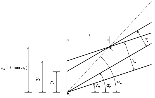

Figure 10. Computing the inclination angle of moiré lines as a function of inclination angles of the base layer and revealing layer lines
From Figure 10 we deduce the following two equations:

From these equations we deduce the equation for computing the inclination of moiré lines as a function of the inclinations of the base layer and the revealing layer lines:
Table 1 shows the moiré lines’ inclinations for several degrees of the revealing layer inclination, for the base layer inclination fixed to 30 degree, with a base layer period equal to 6 units, and with a revealing layer period equal to 5.5 units. The table shows that when the inclination of the lines of the revealing layer is the same as the inclination of the lines of the base layer, the inclination of moiré lines is also identical to the layer lines’ inclination.
Table 1. Inclinations of moiré lines of the superposition image for the base layer lines inclination equal to 30 degrees and for the revealing layer lines inclination from 25 to 35 degrees:
25 -37.06 26 -26.48 27 -13.31 28 1.70 29 16.74 30 30.00 31 40.68 32 48.93 33 55.26 34 60.16 35 64.01
![]()
![]()

For the same set of parameters, the bold curve of Figure 11 represents the moiré line inclination degree as a function of the revealing layer line inclination. The two other curves correspond to cases, when the base layer inclination is equal to 20 and 40 degrees correspondingly. The circle marks correspond to the points where both layers’ lines inclinations are equal, and the moiré lines inclination also become the same.
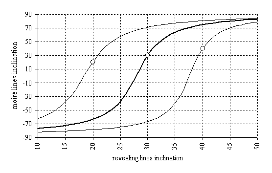
Figure 11. Moiré lines inclination as a function of the revealing layer lines inclination for the base layer lines inclination equal to 30 degrees [xls]
4.3.2. Deducing the known formulas from our equations
The periods ![]() ,
, ![]() , and
, and ![]() used in the literature
are computed as follows (see Figure 10):
used in the literature
are computed as follows (see Figure 10):
|
|
From here, using equation (4.6) we deduce the well known formula for the angle of
moiré lines [Amidror00a]:

Recall from trigonometry the
following simple formulas:
From equations (4.8) and (4.9) we have:


From equations (4.2) and (4.7) we have:
From
equations (4.10) and (4.11) we deduce the second well known formula for the
period ![]() of moiré lines:
of moiré lines:

Recall from trigonometry that:
In the
particular case when ![]() , taking in account equation (4.13), equation (4.12) is further reduced into well known formula:
, taking in account equation (4.13), equation (4.12) is further reduced into well known formula:

Still for the case when ![]() , we can temporarily assume that all angles are
relative to the base layer lines and rewrite equation (4.8) as follows:
, we can temporarily assume that all angles are
relative to the base layer lines and rewrite equation (4.8) as follows:

Recall from trigonometry that:
Therefore from equations (4.15) and (4.16):
|
|
(4.17) |
Now for the case when the revealing layer lines do not represent the
angle zero:
|
|
(4.18) |
We obtain the well known formula [Amidror00a]:
Equations
(4.8) and (4.12) are the general case formulas known in the
literature, and equations (4.14) and (4.19) are the formulas for rotation of identical patterns
with parallel lines (i.e. the case when ![]() ) [Amidror00a], [Nishijima64a], [Oster63a], [Morse61a].
) [Amidror00a], [Nishijima64a], [Oster63a], [Morse61a].
Assuming
in the well known equation (4.8) that ![]() , Figure
12 shows the charts of the moiré lines’ degree as a
function of the revealing layer’s rotation degree for different values of
, Figure
12 shows the charts of the moiré lines’ degree as a
function of the revealing layer’s rotation degree for different values of ![]() .
.
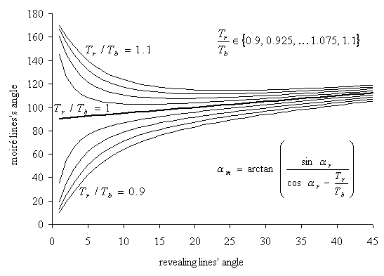
Figure 12. Moiré lines inclination as a function of the rotation degree of the revealing layer [xls]
Only for the case when ![]() (the bold curve) the
rotation of moiré lines is linear with respect to the rotation of the revealing
layer. Comparisons of Figure
12 and Figure
11 show the significant difference between shearing
(i.e. inclination of lines) and rotation of the revealing layer pattern.
(the bold curve) the
rotation of moiré lines is linear with respect to the rotation of the revealing
layer. Comparisons of Figure
12 and Figure
11 show the significant difference between shearing
(i.e. inclination of lines) and rotation of the revealing layer pattern.
4.3.3. The revealing lines inclination as a function of the superposition image’s lines inclination
From equation (4.6) we can deduce the equation for computing the revealing
layer line inclination ![]() for a given base layer
line inclination
for a given base layer
line inclination ![]() , and a desired moiré line inclination
, and a desired moiré line inclination ![]() :
:

The increment of the tangent of revealing lines’
angle (![]() ) relatively to the tangent of the base layer lines’ angle
can be expressed, as follows:
) relatively to the tangent of the base layer lines’ angle
can be expressed, as follows:

According to equation (4.4), ![]() is the inverse of the optical
acceleration factor, and therefore equation (4.21) can be rewritten as follows:
is the inverse of the optical
acceleration factor, and therefore equation (4.21) can be rewritten as follows:
Equation (4.22) shows that relative to the tangent of the base layer lines’ angle, the increment of the tangent of the revealing layer lines’ angle needs to be smaller than the increment of the tangent of the moiré lines’ angle, by the same factor as the optical speedup.
For any given base layer line inclination,
equation (4.20) permits us to obtain a desired moiré line inclination
by properly choosing the revealing layer inclination. In Figure 7 we showed an example where the curves of layers
follow an identical inclination pattern forming a superposition image with the same
inclination pattern. The inclination degrees of the layers’ and moiré lines
change along the horizontal axis according the following sequence of
alternating degree values (+30, –30, +30, –30, +30). In Figure 13 we obtained the same superposition pattern as in Figure 7, but the base layer consists of straight lines
inclined by –10 degrees. The revealing pattern of Figure 13 is computed by interpolating the curves into connected
straight lines, where for each position along the horizontal axis, the
revealing line’s inclination angle is computed as a function of ![]() and
and ![]() , according to equation (4.20). Figure
13 demonstrates what is already expressed by equation (4.22): the difference between the inclination patterns of
the revealing layer and the base layer are several times smaller than the
difference between the inclination patterns of moiré lines and the base layer
lines.
, according to equation (4.20). Figure
13 demonstrates what is already expressed by equation (4.22): the difference between the inclination patterns of
the revealing layer and the base layer are several times smaller than the
difference between the inclination patterns of moiré lines and the base layer
lines.
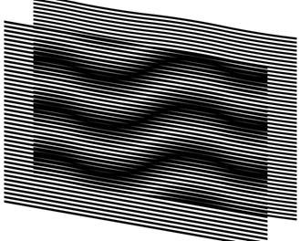
Figure 13. The base layer with inclined straight lines, the revealing layer computed so as to form the desired superposition image [eps], [png]
Another example forming the same superposition patterns as in Figure 7 and Figure 13 is shown in Figure 14. Note that in Figure 14 the desired inclination pattern (+30, –30, +30, –30, +30) is obtained using a base layer with an inverted inclination pattern (–30, +30, –30, +30, –30).
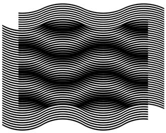
Figure 14. A superposition image, where the base layer and moiré curves are mirrored relatively to the horizontal axis [eps], [png]
The GIF animation of Figure 15 shows a superposition image with a constant inclination pattern of moiré lines (+30, –30, +30, –30, +30) for modifying pairs of base and revealing layers. The base layer inclination pattern gradually changes and the revealing layer inclination pattern correspondingly adapts such that the superposition image’s inclination pattern remains the same.

Figure 15. The revealing, base, and superposition images, where the base layer inclination pattern gradually changes, and the revealing layer correspondingly adapts such that the superposition image’s inclination pattern remains the same [ps], [tif], [gif]
5. Superposition of periodic circular patterns
5.1. Superposition of circular periodic patterns with radial lines
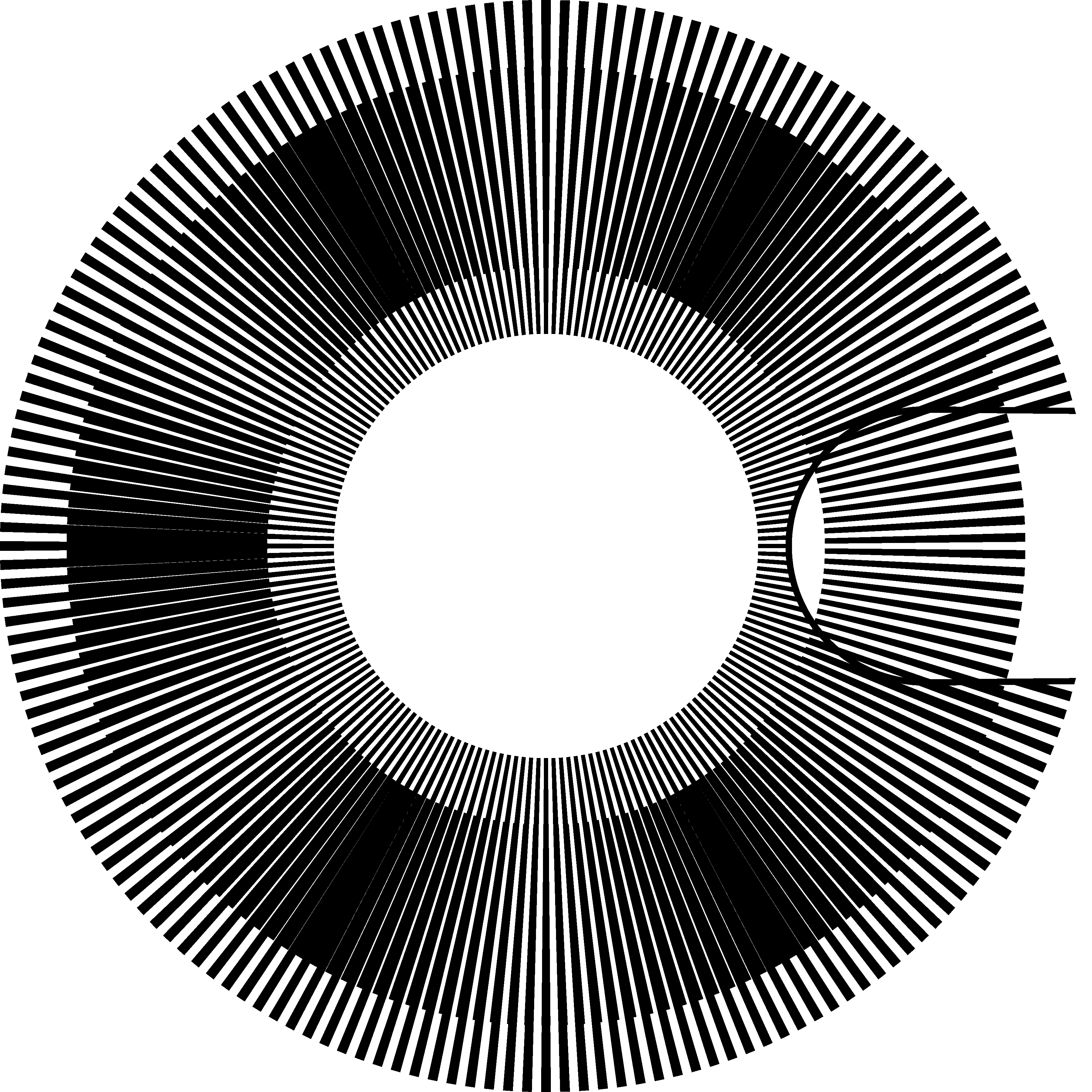
Similarly to layer and moiré patterns comprising parallel lines (see Figure 1, Figure 2, and Figure 3), concentric superposition of dense periodic layer patterns comprising radial lines forms magnified periodic moiré patterns also with radial lines.
Figure
16 is the counterpart of Figure 1, where the horizontal axis is replaced by the radius
and the vertical axis by the angle. Full circumferences of layer patterns are equally
divided by integer numbers of radial lines. The number of radial lines of the
base layer is denoted as ![]() and the number of
radial lines of the revealing layer is denoted as
and the number of
radial lines of the revealing layer is denoted as ![]() .
.
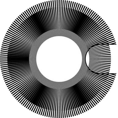
Figure 16. Superposition of two layers with regularly spaced radial segments (a portion of the revealing layer is cut out to show a part of the base layer in the background) [eps], [png]
The periods ![]() and
and ![]() denote the angles
between the central radial axes of adjacent lines. Therefore:
denote the angles
between the central radial axes of adjacent lines. Therefore:
According to equations (5.1), equation (4.2) can be rewritten as follows:
Therefore the number of moiré radial lines ![]() corresponds to the
difference between the numbers of layer lines:
corresponds to the
difference between the numbers of layer lines:
If in the layer patterns, the full circumferences are divided by integer numbers of layer lines, the circumference of the superposition image is also divided by an integer number of more lines.
Radial lines in Figure 16 have constant angular thickness, giving them the
forms of segments, thick at their outer ends and thin at their inner ends. The
thickness of radial lines affects the overall darkness of the superposition
image and the width of moiré bands, but there is no impact on other factors,
such as period of superposition pattern (i.e. values of ![]() and
and ![]() ). In our examples the angular thicknesses of layer lines are
equal to the layer’s half-period, i.e. the thickness of the base layer lines is
equal to
). In our examples the angular thicknesses of layer lines are
equal to the layer’s half-period, i.e. the thickness of the base layer lines is
equal to ![]() and the thickness of
the revealing layer lines is
and the thickness of
the revealing layer lines is ![]() .
.
The optical speedup factor of equation (4.4) can be rewritten by replacing the periods![]() and
and ![]() by their expressions from equations (5.1):
by their expressions from equations (5.1):
The values ![]() and
and ![]() represent the angular
speeds. The negative speedup signifies a rotation of the superposition image in
a direction inverse to the rotation of the revealing layer. Considering (5.3), the absolute value of the optical speedup factor is:
represent the angular
speeds. The negative speedup signifies a rotation of the superposition image in
a direction inverse to the rotation of the revealing layer. Considering (5.3), the absolute value of the optical speedup factor is:

In Figure 16, the number of radial lines of the revealing layer is equal to 180, and the number of radial lines of the base layer is 174. Therefore, according to equations (5.4) and (5.3), the optical speedup is equal to 30, confirmed by the two images (a) and (b) of Figure 17, and the number of moiré lines is equal to 6, confirmed by the image of Figure 16.
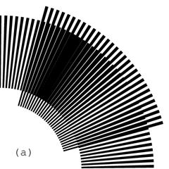
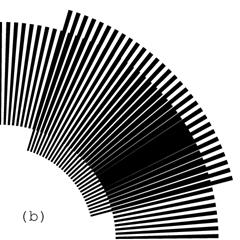
Figure 17. Rotation of the revealing layer by 1 degree in the clockwise direction rotates the optical image by 30 degrees in the same direction [eps (a)], [png (a)], [eps (b)], [png (b)]
Figure 18 shows a GIF animation of the superposition image of Figure 16, where the revealing layer slowly rotates in the clockwise direction.
Figure 18. GIF animation of the superposition image of the layers with periodic radial lines, where the revealing layer slowly rotates clockwise [ps], [tif], [gif]
5.2. Superposition of circular patterns with radial curves
In
circular periodic patterns curved radial lines can be constructed using the
same reference sequences of inclination degrees as used in section 4.3 for curves of Figure
7. The inclination angle at any point of the radial
curve corresponds to the angle between the curve and the axis of the radius
passing through the current point. Thus inclination angle 0 corresponds to straight
radial lines as shown in Figure
16. With the present notion of inclination angles for ![]() ,
, ![]() , and
, and ![]() , equations (4.6) and (4.20) are applicable for circular patterns without
modifications.
, equations (4.6) and (4.20) are applicable for circular patterns without
modifications.
Curves can be constructed incrementally with a
constant radial increment equal to ![]() . Figure
19 shows a segment of a curve, marked by a thick line,
which has an inclination angle equal to
. Figure
19 shows a segment of a curve, marked by a thick line,
which has an inclination angle equal to ![]() .
.
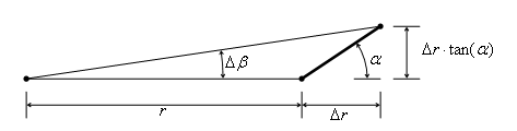

Figure 19. Constructing a curve in a polar coordinate system with a desired inclination
While constructing the curve, the current
angular increment ![]() must be computed so as
to respect the inclination angle
must be computed so as
to respect the inclination angle ![]() :
:
Figure
20 shows a superposition of layers with curved radial
lines. The inclination of curves of both layers follows an identical pattern
corresponding to the following sequence of degrees (+30, –30, +30, –30, +30). Layer
curves are iteratively constructed with increment pairs ![]() computed according to
equation (5.6). Since the inclination patterns of both layers of Figure 20 are identical, the moiré curves also follow the same
pattern.
computed according to
equation (5.6). Since the inclination patterns of both layers of Figure 20 are identical, the moiré curves also follow the same
pattern.
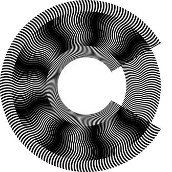
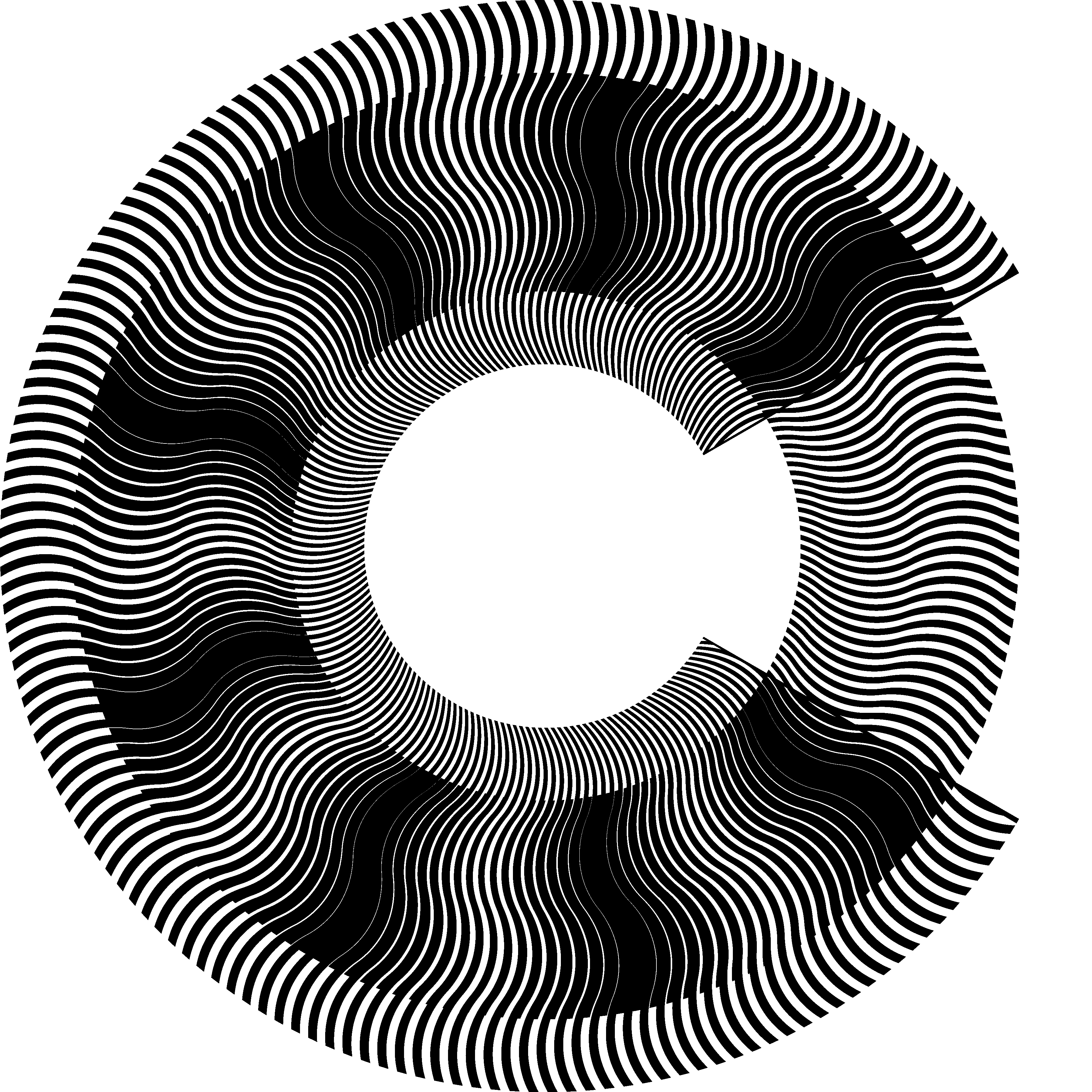
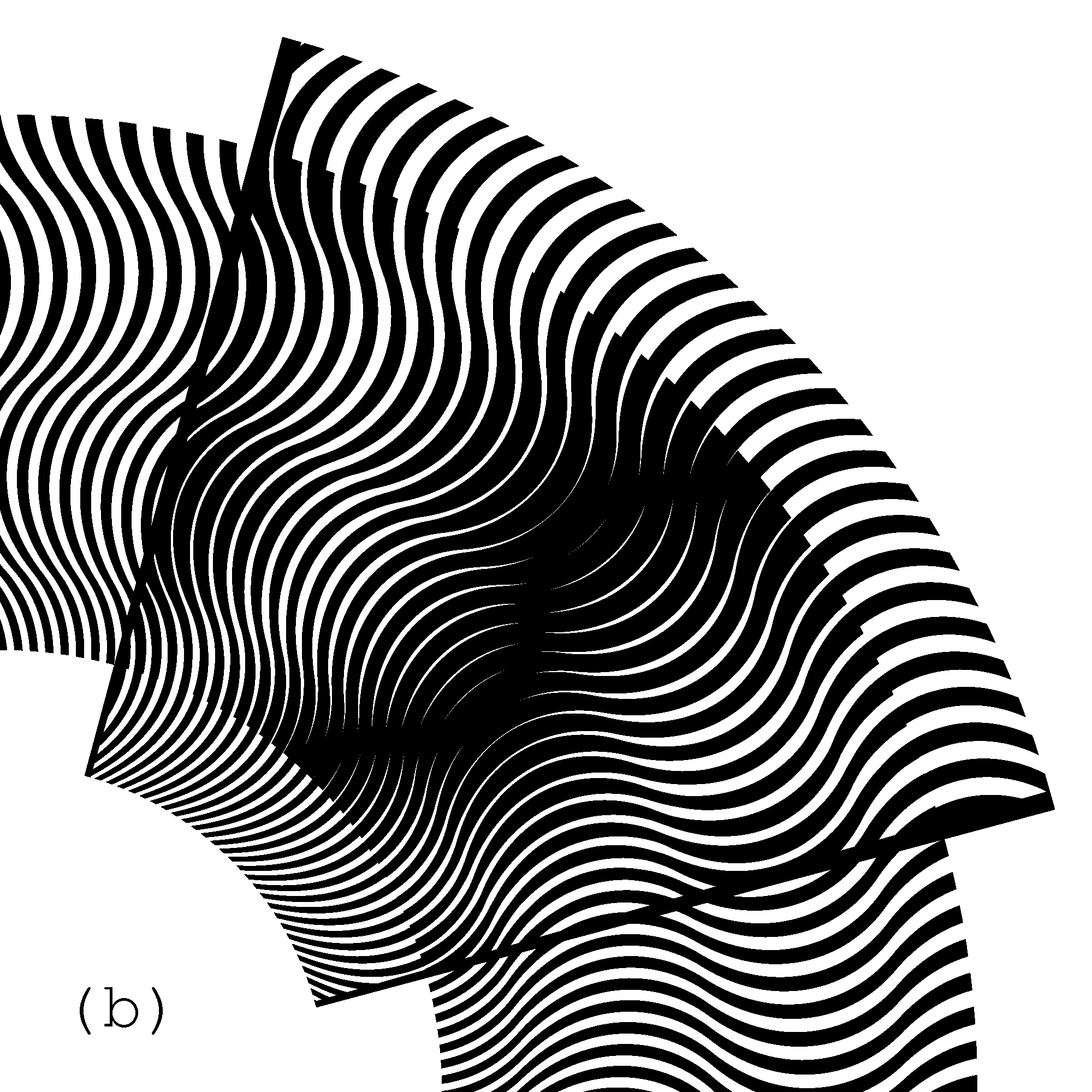
Figure 20. Superposition of layers in a polar coordinate system with identical inclination patterns of curves corresponding to (+30, –30, +30, –30, +30); a portion of the revealing layer is cut away exposing the base layer in the background [eps], [png], multi-page [tif], [gif]
Similarly to examples of Figure 7, Figure 13, and Figure 14, where the same moiré pattern is obtained by superposing different pairs of layer patterns, the circular moiré pattern of Figure 20 can be analogously obtained by superposing other pairs of circular layer patterns. Taking into account equations (5.1), equations (4.6) and (4.20) can be rewritten as follows:
|
|
(5.7) |

Thanks to equation (5.8), other pairs of layer patterns can be created (see Figure 21) which produce the same superposition image as in Figure 20. In the first image (a) of Figure 21, the base layer lines are straight. In the second image (b), the base layer lines inclination pattern is reversed with respect to the moiré lines.
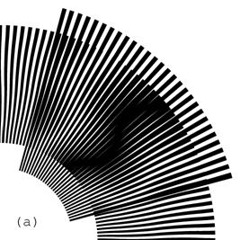
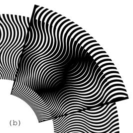
Figure 21. Superposition images with identical inclination pattern (+45, –45, +45, –45, +45) of moiré curves, where in one case the base layer comprise straight radial segments, and in the second case the base layer comprise curves which are the mirrored counterparts of the resulting moiré curves [eps (a)], [png (a)], [eps (b)], [png (b)]
Figure 22 shows an animation, where the moiré curves of the superposition image are always the same, but the inclination pattern of the base layer curves gradually alternates between the following two mirror patterns (+45, –45, +45, –45, +45), and (–45, +45, –45, +45, –45). For each instance of the animation, the revealing layer lines are computed according to equation (5.8) in order to constantly maintain the same moiré pattern.

Figure 22. Animation of the superposition image, where the base layer lines gradually change their inclination pattern from (+45, –45, +45, –45, +45) to (–45, +45, –45, +45, –45) [eps], [tif], [gif]
Equations (5.4) and (5.3) remain valid for patterns with curved radial lines. In Figure 20 there are 180 curves in the revealing layer and 171 curves in the base layer. Therefore optical speedup factor according to equation (5.4) is equal to 20, and the number of moiré curves according to equation (5.3) is equal to 9, as seen in the superposition image of Figure 20.
6. Conclusions
We redeveloped the most important formulas for computing the periods, inclination angles of moiré patterns, and the velocities of optical shapes.
Instead of using the well known equations, we represent the case of inclined patterns such that equations (4.2), (4.3), and (4.4) for linear patterns and their counterparts (5.3), (5.5), and (5.4) for circular patters, remain valid in their simple forms. In our equations, the p values represent the periods along the axis of the movement of the revealing layer.
In section 4.3.2 we compared our formulas with the formulas known in the literature.
7. References
[Amidror00a] Isaac Amidror, The Theory of the Moiré Phenomenon, Kluwer Academic Publisher, 2000 [CH], [US]
[Amidror03a] Isaac Amidror, “Glass patterns in the superposition of random line gratings”, Journal of Optics A: Pure and Applied Optics, 28 March 2003, pp. 205-215 [CH], [US]
[Nishijima64a] Y. Nishijima and G. Oster, “Moiré patterns: their application to refractive index and refractive index gradient measurements”, Journal of the Optical Society of America, Vol. 54, No. 1, January 1964, pp. 1-5 [CH], [US]
[Oster63a] G. Oster and Y. Nishijima, “Moiré patterns”, Scientific American, Vol. 208, May 1963, pp. 54-63
[Sciammarella62a] C. A. Sciammarella and A. J. Durelli, “Moiré fringes as a means of analyzing strains”, American Society of Civil Engineers, Vol. 127, Part I, 1962, pp. 582-587 [CH], [US]
[Morse61a]
8. Table of figures
Figure
2. Superposition of two layers consisting of horizontal parallel lines [eps],
[tif], [png]
Figure
5. GIF animation of the slow vertical movement of the revealing layer [ps],
[gif], [tif]
Figure
12. Moiré lines inclination as a function of the rotation degree of the
revealing layer [xls]
Figure
19. Constructing a curve in a polar coordinate system with a desired inclination
9. Links
(070212) Random moiré [CH], [US]
(070227) Random line moiré [CH], [US]
(070306) This web site: periodic line moiré patterns and optical speedup [CH], [US]
Format [doc], [pdf], [htm], [htm (ms)]
* * *