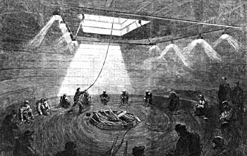
Figure 1. Loading the transatlantic cable into the ‘Great Eastern’ in 1865................ 1
Figure 2. Diagrams from the 51-page report of Paul Baran to the U.S. Air Force, 1964 2
Figure 3. Kidney blood filtering in the human organism............................................ 3
Figure 4. Pulmonary circuit of the human organism.................................................. 3
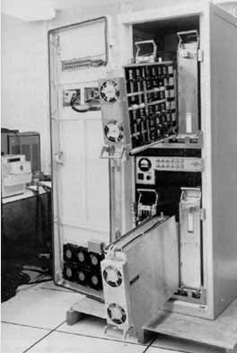
Figure 5. One of the first Interface Message Processor (IMP) of ARPANET connecting UCLA with SRI in August 1969 4
Figure 6. Packet switching network: packets are entirely stored at each intermediate switch and then only forwarded to the next switch................................................................................................ 5
Figure 7. Wormhole or cut-through routing network: a packet is “copied” through the communication path from the source directly to the destination without being stored in any intermediate switch................... 6
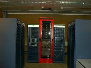
Figure 8. The final generation of the Swiss-Tx supercomputer in June 2001........... 11
Figure 9. File Striping........................................................................................... 12
Figure 10. SFIO integration into MPI-I/O.............................................................. 14
Figure 11. Distribution of a striped file across subfiles............................................. 16
Figure 12. Disk access optimization........................................................................ 17
Figure 13. Comparison of the optimized write access with a generic write access on the scale of the file striping granularity (3 I/O nodes, 1 compute node, global file size is 660 Mbytes)............................ 18
Figure 14. Comparison of the optimized multi-block write access with a generic write access on the scale of the user memory fragmentation (Fast Ethernet, stripe unit size is 1005 bytes).................................... 18
Figure 15. SFIO functional architecture.................................................................. 19
Figure 16. Aggregate throughput of Fast Ethernet as a function of the number of the contributing nodes 21
Figure 17. SFIO architecture on Swiss-T1............................................................. 22
Figure 18. SFIO/MPICH all-to-all I/O performance for a 200 bytes stripe size....... 22
Figure 19. Aggregate throughput of TNET as a function of the number of the contributing nodes 23
Figure 20. The Swiss-T1 network interconnection topology.................................... 24
Figure 21. SFIO all-to-all I/O performance on TNET............................................. 25
Figure 22. The use of derived datatypes in MPI-I/O interface................................. 26
Figure 23. The recursive construction of derived datatypes in MPI (“Contiguous” is a derived datatype obtained by joining a repeated number of times another datatype, which in its turn can be fragmented).... 27
Figure 24. MPI-I/O implementation requires a method for retrieving the fragmentation patterns of opaque MPI derived datatypes 28
Figure 25. A reverse engineering method for discovery the fragmentation pattern of an opaque datatype built by the user 29
Figure 26. Isolated implementation of a portable MPI-I/O interface functional on any MPI-1 implementation 30
Figure 27. In the first layer the flow is equally split across two paths, two links of which, marked by thick dashes, are the bottlenecks. 35
Figure 28. The second layer minimizes to 1/3 the maximal load of the remaining seven links and identifies three bottlenecks. 35
Figure 29. The third layer minimizes to 1/4 the maximal load of the remaining four links and identifies two bottlenecks. 35
Figure 30. Routing pattern of layer 10 built by the capillary routing algorithm on a network sample with 150 nodes 36
Figure 31. Initial problem with one source and one sink node.................................. 37
Figure 32. Maximize the flow, fix the new flow-out coefficients at the nodes and find the bottleneck links (layer 1, ) 37
Figure 33. Remove the bottleneck links from the network and adjust the flow-out coefficients at the adjacent nodes 37
Figure 34. Maximize the flow in the new sub-problem, fix the new flow-out coefficients at the nodes and find the new bottlenecks (layer 2, )....................................................................................................... 37
Figure 35. Again remove the bottleneck links from the network and adjust correspondingly the flow-out coefficients at the adjacent nodes......................................................................................................... 37
Figure 36. Maximize the flow in the obtained new problem, fixing the new resulting flow-out coefficients at the nodes and find the new bottlenecks (layer 3, )............................................................................. 37
Figure 37. An example of a bounded multi-source/multi-sink problem (obtained during construction of the capillary routing from a network with one source and one destination node)...................................... 39
Figure 38. A max-flow solution with the flow increase factor of 4/3, containing four maximally loaded candidate links {a, b, d, e} 39
Figure 39. Cost reduction applied to four fully loaded links of Figure 38 reduces the load of suspected link d, and the suspect list is now {a, b, e}................................................................................................ 39
Figure 40. Cost reduction applied to the three fully loaded links of Figure 39 reduces the load of another suspected link a, and the true bottleneck links are {b, e}.................................................................... 39
Figure 41. Decrease of the number of suspected links during the bottleneck hunting loop of each of 10 capillary routing layers 40
Figure 42. Transmission rate increase factor as a function from the packet loss rate ( ) 43
Figure 43. Average ROR as a function from the capillary routing layer..................... 44
Figure 44. Average ROR computed assuming real-time streaming (the group of curves above) and off-line streaming (the group below) 45
Figure 45. Yearly fractions of IEEE publications related to Parallel I/O.................... 47
* * *