List of Figures

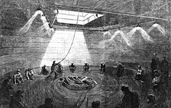
Figure 1.	Loading the transatlantic cable into the ‘Great Eastern’ in 1865	........... 1
Figure 2.	Diagrams from the 51-page report of Paul Baran to the U.S. Air Force, 1964	........... 2
Figure 3.	Kidney blood filtering in the human organism	........... 3
Figure 4.	Pulmonary circuit of the human organism	........... 4
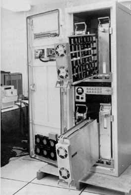
Figure 5.	One of the first Interface Message Processor (IMP) of ARPANET connecting UCLA with SRI in August 1969	........... 5
Figure 6.	Packet switching network: packets are entirely stored at each intermediate switch and only then forwarded to the next switch	........... 5
Figure 7.	Wormhole or cut-through routing network: a packet is “copied” through the communication path from the source directly to the destination without being stored in any intermediate switch	........... 6
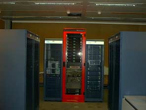
Figure 8.	Swiss-Tx supercomputer in June 2001	......... 13
Figure 9.	File Striping	......... 14
Figure 10.	SFIO integration into MPI-I/O	......... 16
Figure 11.	Distribution of a striped file across subfiles	......... 18
Figure 12.	Disk access optimization	......... 19
Figure 13.	Comparison of the optimized write access with a non-optimized write access as a function of the file striping granularity (3 I/O nodes, 1 compute node, global file size is 660 Mbytes)	......... 20
Figure 14.	Comparison of the optimized multi-block write access with corresponding separate non-optimized single block accesses (Fast Ethernet, stripe unit size is 1005 bytes, 7 I/O nodes)	......... 20
Figure 15.	SFIO functional architecture	......... 21
Figure 16.	Aggregate throughput of Fast Ethernet as a function of the number of contributing nodes	......... 24
Figure 17.	SFIO architecture on Swiss-T1	......... 24
Figure 18.	SFIO/MPICH all-to-all I/O performance for a 200 byte stripe size	......... 25
Figure 19.	Aggregate throughput of TNET as a function of the number of the contributing nodes	......... 25
Figure 20.	The Swiss-T1 network interconnection topology	......... 26
Figure 21.	SFIO all-to-all I/O performance on TNET	......... 27
Figure 22.	The use of derived datatypes in MPI-I/O interface	......... 29
Figure 23.	The recursive construction of derived datatypes in MPI (“Contiguous” is a derived datatype obtained by repeatedly joining another datatype which in turn can be fragmented)	......... 29
Figure 24.	The MPI-I/O implementation requires a method for retrieving the fragmentation patterns of opaque MPI derived datatypes	......... 30
Figure 25.	A reverse engineering method for discovery the fragmentation pattern of an opaque datatype built by the user	......... 31
Figure 26.	Isolated implementation of a portable MPI-I/O interface functional on any MPI-1 implementation	......... 32
Figure 27.	Wavelength routing in optical layer	......... 40
Figure 28.	A simple network sample (pictograms)	......... 42
Figure 29.	The pictograms representing the 25 transfers from all sending nodes to all receiving nodes of the network of Figure 28	......... 43
Figure 30.	Example of a traffic comprising 25 transfers carried out over the network shown in Figure 28	......... 45
Figure 31.	An initial category before fission, where symbol , represents any transfer that is in congestion with and symbol represents any transfer which is simultaneous with	......... 48
Figure 32.	Fission of the category of Figure 31 into its positive and negative sub categories.	......... 48
Figure 33.	Proportion of the number of transfers within a skeleton, compared with the number of transfers of the corresponding traffic	......... 50
Figure 34.	Search space reduction obtained by idle+skeleton+blank optimization steps	......... 52
Figure 35.	Time frames of a liquid schedule of the collective traffic shown in Figure 30	......... 53
Figure 36.	There exists a traffic of three transmissions across this network that has no team and therefore no liquid schedule	......... 54
Figure 37.	A traffic consisting of thee transmissions to be carried across the network shown in Figure 36	......... 54
Figure 38.	Liquid schedule construction tree: denotes a reduced subtraffic at the layer of the tree and denotes a candidate for the time frame ; the operator applied to a subtraffic yields the set of all possible candidates for a time frame	......... 55
Figure 39.	Architecture of the Swiss-T1 cluster supercomputer interconnected by a high performance wormhole switch fabric	......... 58
Figure 40.	For a given number of contributing nodes all possible allocation of nodes yielding different liquid throughputs	......... 59
Figure 41.	The 362 topologies of Figure 40 yielding different liquid throughput values placed along one axis, sorted first by the number of contributing nodes and then by their liquid throughputs	......... 60
Figure 42.	Theoretical liquid throughput and measured round-robin schedule throughput for 362 network sub topologies.	......... 61
Figure 43.	Predicted liquid throughput and measured throughput according to the computed liquid schedule	......... 61
Figure 44.	In the first layer the flow is equally split across two paths. Two of their links, marked by thick dashes, are the bottlenecks.	......... 66
Figure 45.	The second layer minimizes to 1/3 the maximal load of the remaining seven links and identifies three bottlenecks.	......... 66
Figure 46.	The third layer minimizes to 1/4 the maximal load of the remaining four links and identifies two bottlenecks.	......... 66
Figure 47.	Routing pattern of layer 10 built by the capillary routing algorithm on a network sample with 180 nodes [zip]	......... 66
Figure 48.	Initial problem with one source and one sink node	......... 67
Figure 49.	Maximize the flow, fix the new flow-out coefficients at the nodes and find the bottleneck links (layer 1, )	......... 67
Figure 50.	Remove the bottleneck links from the network and adjust the flow-out coefficients at the adjacent nodes	......... 67
Figure 51.	Maximize the flow in the new sub-problem, fix the new flow-out coefficients at the nodes and find the new bottlenecks (layer 2, )	......... 68
Figure 52.	Again remove the bottleneck links from the network and adjust correspondingly the flow-out coefficients at the adjacent nodes	......... 68
Figure 53.	Maximize the flow in the obtained new problem, fixing the new resulting flow-out coefficients at the nodes and find the new bottlenecks (layer 3, )	......... 68
Figure 54.	An example of a bounded multi-source/multi-sink problem (obtained during construction of the capillary routing from a network with one source and one destination node)	......... 69
Figure 55.	A max-flow solution with the flow increase factor of 4/3, containing four maximally loaded candidate links {a, b, d, e}	......... 69
Figure 56.	The cost reduction applied to the four fully loaded links of Figure 55 reduces the load of suspected link d, and the bottleneck candidate list is now {a, b, e}.	......... 70
Figure 57.	The cost reduction applied to the three fully loaded links of Figure 56 reduces the load of another suspected link a. The true bottleneck links are {b, e}.	......... 70
Figure 58.	Decrease of the number of suspected links during the bottleneck hunting loop at each of the 10 capillary routing layers	......... 70
Figure 59.	Transmission rate increase factor as a function of the packet loss rate ()	......... 74
Figure 60.	Average ROR metric as a function of the capillary routing layer	......... 76
Figure 61.	Average ROR metric computed assuming real-time streaming (the group of curves above) and off-line streaming (the group below)	......... 76
Figure 62.	Congestion graph corresponding to the traffic pattern of Figure 29 across the network of Figure 28: the vertices of the graph represent the 25 transfers, the edges represent congestions between the transfers	......... 85
Figure 63.	Number of edges in the 362 congestion graphs corresponding to the traffic patterns of Figure 40 and Figure 41	......... 86
Figure 64.	Loss in throughput induced by schedules computed with the DSatur heuristic algorithm	......... 87
Figure 65.	Running times for computing liquid schedules with the MILP Cplex method and with the liquid schedule construction algorithm	......... 90
Figure 66.	The overall measured throughputs of hundreds of different traffic patterns carried out according to a liquid schedule and according to a topology unaware schedule	......... 98
Figure 67.	The probability that the interarrival time between two consecutive failures in a Poisson process is less than a given time, ,	....... 100

* * *